Improving Delivery Performance of Construction Manufacturing Using Machine Learning
ACM Subject Categories
Applied computing~Operations research~Industry and manufacturing~Command and controlApplied computing~Operations research~Industry and manufacturing~Supply chain managementComputing methodologies~Machine learning~Learning paradigms~Reinforcement learning
Keywords
- Construction Manufacturing
- Deep Artificial Neural Networks
- Delivery Performance
- Precast Reinforced Concrete Components
- Reinforcement Learning
Abstract
This paper is concerned with the development, testing, and optimization of a machine learning method for controlling the production of precast reinforced concrete components. A discussion is given identifying the unique challenges associated with achieving production efficiency in the construction industry, namely: uncertain and sporadic demand for work; high customization of the design of components; a need to produce work to order; and little prospect for stockpiling work. This is followed by a review of the methods available to tackle this problem, which can be divided into search-based techniques (such as heuristics) and experience-based techniques (such as artificial neural networks). A model of an actual factory for producing precast reinforced concrete components is then described, to be used in the development and testing of the controller. A reinforcement learning strategy is proposed for training a deep artificial neural network to act as the control policy for this factory. The ability of this policy to learn is evaluated, and its performance is compared to that of a rule-of-thumb and a random policy for a series of testing production runs. The reinforcement learning method developed an effective and reliable policy that significantly outperformed the rule-of-thumb and random policies. An additional series of experiments were undertaken to further optimize the performance of the method, ranging the number of input variables presented to the policy. The paper concludes with an indication of proposed future research designed to further improve performance and to extend the scope of application of the method.
Introduction
Factory-based construction manufacturing has the potential to overcome many of the inefficiencies of traditional on-site methods. However, achieving production efficiency in a construction factory is usually more challenging than for other manufacturing industries. This is because construction work does not lend itself to the methods of mass production. Work arrives in batches at irregular intervals with large fluctuations in demand, the work can be diverse in design both between and within batches, and the products are rarely reproduced. Consequently, work has to be made to order with little or no potential for stockpiling, and with large variations in the demand for productive resources.
Controlling construction operations (such as selecting the next job in a queue to be processed) is unlikely to be achieved optimally by simple manually crafted rules, given the complexities of construction demand. A more sophisticated rule system, taking into account a wide range of system situations and outcomes, is required. A promising approach to this problem is machine learning (ML), whereby an artificial intelligence (AI) agent uses a deep artificial neural network (DANN) to control operations. These agents would act like an advisor in a human-in-the-loop system, or as a controller in an automated system, generating solutions whenever an operational decision is required.
The use of AI-based decision agents to control operations in construction is limited. Shitole et al. (2019) developed an AI agent for optimizing a simulated earth-moving operation based on artificial neural networks (ANNs) trained using reinforcement learning (RL), and found it outperformed previously published manually crafted heuristics. RL is a broad class of learning techniques based on discovery and rewards that has demonstrated much success in recent years (Sutton & Barto, 2018). Their earth-moving system comprised two excavators serving a fleet of dump-trucks. The function of the AI agent was to direct the trucks to one or other of the excavators at a junction in the return road, with the goal of optimizing the overall production rate of the system. An issue with this approach to process control is its lack of extensibility. That is, the AI agent can only be applied to the earth-moving system considered in the study. Applying the AI agent to a new situation with a different site layout and/or equipment combination would require retraining. Although this could be achieved prior to the start of the new construction operation, it would nevertheless be a significant burden on pre-construction planning. Clearly, there is a need for more work in the area of ANN extensibility.
An alternative application area to site-based construction, with more immediate application given current AI technology, is factory centered manufactured construction. In this situation, the life-span of an AI agent should be relatively long, lasting at least until any reconfiguration of the factory system is required or a change occurs in its operating environment. This study is focused on factory-based construction manufacture, specifically for precast reinforced concrete (PRC) component production.
Optimization of customized PRC component production has been considered by several researchers (Leu & Hwang, 2001; Chan & Hu, 2002; Benjaoran & Dawood, 2005), using genetic algorithms (GAs) to improve production performance. Although the approach was shown to be successful, heuristic search methods such as GAs are computationally expensive. Therefore, they are not well suited to situations where decisions have to be made in real-time.
RL solutions based on a learned model, such as that developed by Shitole et al. (2019), will generate rapid solutions to a decision problem, once trained. A number of authors have applied this method to the control of factory operations (Waschneck et al., 2018; Zhou et al., 2020; Xia et al., 2021) and found results to be promising when compared to more conventional approaches such as rule-of-thumb decision techniques. Unfortunately, applications have been outside construction manufacturing, and therefore do not address many of the challenges of this industry (such as uncertainty in the arrival of jobs, size of the batches, processing time, and design of the products), although Waschneck et al. (2018) did consider some level of product customization within the semiconductor industry.
This paper presents a more detailed analysis and extension to the work by Flood & Flood (2022) published in the proceedings of the 12th International Conference on Simulation and Modeling Methodologies, Technologies and Applications, Lisbon. The Lisbon paper performed a proof-of-concept on the viability of using an RL trained DANN to control factory-based manufacture of PRC components, given the unique demands of the construction industry. This paper goes beyond that proof-of-concept to: (a) model a real PRC component factory using data published by Wang et al. (2018); (b) extend the depth and scope of the performance experiments and their analyses; and, (c) add new research investigating the impact on performance of increasing the choices made available to the DANN-based decision agent.
Factory-Based Production Control
Decision Agents
The future track followed by a construction manufacturing system is determined by both controllable and uncontrollable events. The controllable events provide an opportunity to steer this track along a line that is favorable to the manufacturer, optimizing performance in terms of, say, productivity and/or profit. This is achieved through the selection of an appropriate sequence of decisions wherever options exist. Examples of such decisions include prioritizing jobs in a queue, deciding when to take an item of equipment offline for maintenance, and selecting the number of machines to allocate to a process.
These decisions are made by one or more agents, as illustrated in Figure 1, that operate dynamically throughout the life of the manufacturing system. An agent monitors relevant variables defining the state of the system and its environment, S, (both current and possibly past states, and even predictions about future states) then uses these insights to decide on appropriate future actions to implement. Typically, these actions will concern events in the immediate future (given that the most relevant, accurate, and valuable information is available at the time of the decision) but can also be applied to events later in the future for decisions that have a long lead time, such as the purchase of resources.
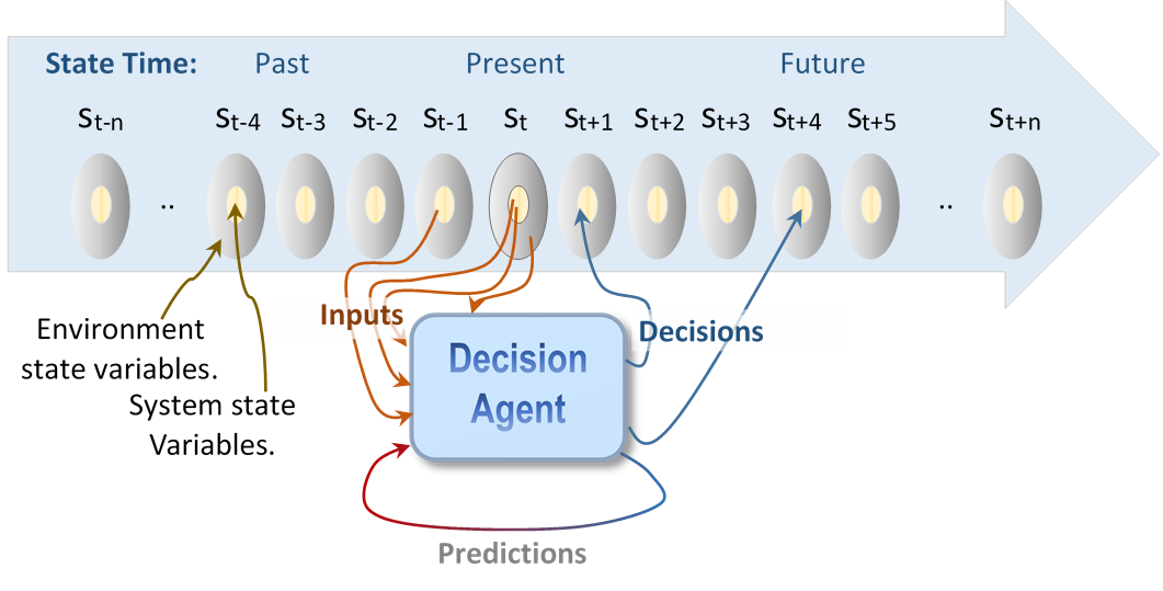
An important dichotomy of decision agents is search-based versus experience-based systems. Search-based agents, which include blind and heuristic methods, use a systematic exploration of the solution space looking for the best action attainable. They tailor a solution to the specific instance of the problem at hand. As such, they may find better optimized solutions than experience-based agents, although that needs to be tested. Search-based agents are also highly extensible, meaning they can be easily adapted to new versions of the problem. A shortcoming is that they can be computationally expensive and thus not suited to situations requiring real-time rapid decision making.
In contrast, experience-based agents, which include rules-of-thumb and ANNs, make decisions based on exposure to similar situations from the past. Once developed, an experience-based agent can output decisions rapidly. However, because the solutions they offer are generic rather than tailored to each situation, their decisions may not be as well optimized as those of search-based agents. Furthermore, experience-based agents tend to lack extensibility; each new version of the problem requires redevelopment of the agent, which in turn requires the acquisition and assimilation of large volumes of new information on system behavior.
A hybrid of these agent types is also possible. For example, an experience-based agent can be used to make the first attempt at a solution and then a search-based agent can be used to improve on this result. Conversely, a search-based agent could be used to acquire examples for development of an experience-based agent.
A longer term objective for this study is to quantify and compare the benefits of search-based and experience-based approaches to controlling construction production systems. This paper, however, focuses on experience-based approaches applied to factory-based construction manufacturing. Two experience-based methods are considered, a rule-of-thumb and a DANN, representing two extremes in functional complexity. DANNs are variants of ANNs that include multiple hidden layers or recursion between units. The additional structure offers a corresponding increase in functional complexity, although model development has additional challenges. Although a DANN is an experience-based approach, its development will involve the use of search techniques to gather good training solutions, specifically using RL techniques. The rule-of-thumb and the DANN are compared to a random decision making method used as a performance benchmark.
DANN Development Strategies
For a construction manufacturing environment, optimal solutions to decision problems are not easily attained a priori or from direct observation of the real system. This excludes the direct use of supervised training techniques for development of the DANN. There are many ways around this problem, including using a strategy of hindsight whereby the agent explores alternative decision tracks in a simulation environment, then selects those that are most successful, effectively learning by trial-and-error.
For DANNs, there are two broad approaches to hindsight model development. The first is to explore adjustments to the structure and/or weights of the model directly, and to select those that result in a better performing decision track. This is in effect an evolutionary method (see, for example, Iba & Noman (2020), and was the basic strategy investigated by Flood (1989) for selecting sequences for construction jobs in an offline optimization problem. The second approach is to explore adjustments to the output from the model, then to evaluate their impact on the performance of the decision track and to feed this back to the model in a supervised manner. This was the approach adopted for this study, and can be classified as a RL method.
Modeling
A key function of RL is the exploration of alternative decision tracks and their impact on the performance of the system. This experience is used to shape the decisions made by the agent, mapping from system state to action. This mapping is referred to as the decision policy.
In construction production (including factory-based construction manufacturing) it is not practicable to experiment with alternative decision policies using the real system. Construction work is rarely reproduced making it almost impossible to compare the effectiveness of alternative strategies. Artificially reproducing work is also not viable given the cost and time required to manufacture a construction component. One way around this problem is to build a simulation model of the construction production system, and then to use this to experiment with alternative policies. This concept is illustrated in Figure 2, where the blue line represents the historic track taken by the real system, and the orange lines represent alternative future tracks explored by different policies in a simulated version of the system. Information about the real system and its past behavior would be used to develop and validate the simulation model. The information gathered from the simulated system are used to develop and test (validate) the policy, as described in Section 4.
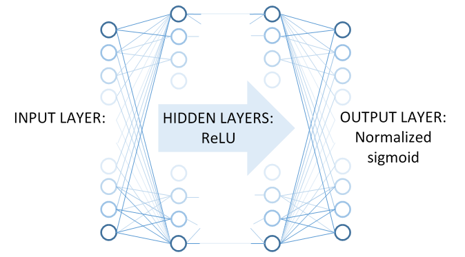
Figure 3 shows a schematic model of the production system considered for this study, representing the manufacture of PRC components such as walls, floors, beams, and column units. The system and its process duration data were obtained from the study published by Wang et al. (2018). This study was chosen because it captures the challenging and unique features of construction manufacturing, namely: In addition, the following assumptions were made about the system: The stochastic time related data used for this study, including their distribution types, are given in Table 1. The dynamics of the system are given by the relative values of these data (rather than by their absolute values) and therefore time units are not included. The triangular distribution was adopted because it is computationally inexpensive and yet provides a versatile way of approximating a wide range of distribution shapes, including those with skew. The control of the system is undertaken by a decision agent as shown in Figure 3. Whenever a vacancy arises at a process, the agent will select a PRC component for processing from the corresponding queue, using its current policy. Three alternative types of policy were considered: The DANN has a layered feedforward structure as shown in Figure 4. The input layer receives both temporal and spatial information about the state of the system and the work to be completed. The input values specify the process durations and the remaining contingencies for the PRC components currently in the queue under consideration. These data are normalized at the input for each process. The location of the values at the input indicates the position in the queue, and the relevant process. An issue with this approach stems from the fact that the structure of the inputs to the DANN is fixed (DANNs are structurally rigid) yet the number of PRC components in the system that need to be evaluated is variable. To get around this, the DANN was designed to allow up to a stipulated number (N) of PRC components to be evaluated in each queue: if the number of PRC components in a queue is less than N then the spare input values are set to 0.0; and if the number of PRC components in a queue is greater than N then only the first N PRC components will be evaluated. Furthermore, the N PRC components evaluated are those with the least contingency, and in this sense the DANN is a hybrid with the rule-of-thumb policy. The value of N used varied between 0 and 30, as detailed in the results, Section 5. The number of hidden layers was set to 6 and the number of hidden units per layer was set to 64. These values were found to have good performance in the DANN training phase (see Section 4.2) in a preliminary search. A more thorough sensitivity analysis ranging these parameters is planned for future work. All hidden units adopted the ReLU (rectified linear unit) activation function due its computational efficiency and avoidance of the vanishing gradient problem (Glorot et al., 2011). The DANNs output layer is where the PRC components are selected from the queues for processing. All output units use a sigmoid activation function, thereby limiting their activation to values between 0.0 and 1.0. The output units correspond a position in the queue. The number of units is equal to N, the number of PRC components to be evaluated in a queue (see Section 3.3.1). The current length of a queue or N, whichever is smallest, determines the number of units that are active. The values generated at the active output units are normalized to sum to 1.0. This allows the output values to be treated as probabilities for selecting PRC components from a queue. The DANN policy has two modes of operation:
Production Simulator

System Variable
Form of Uncertainty
Parameters
Order arrival time
Poisson process
Arrival rate (λ)
Batch size
Discretized triangular distribution
Min
Mode
Max
1
20
100
Rebar durations
Triangular distribution
Min
Mode
Max
120
200
250
Forms durations
Triangular distribution
Min
Mode
Max
130
150
170
Concrete duration
Triangular distribution
Min
Mode
Max
0
50
70
Cure duration
Fixed
~
Strip duration
Triangular duration
Min
Mode
Max
80
100
120
Delivery duration
Triangular distribution
Min
Mode
Max
30
50
70
Contingency time relative to site assembly time
Triangular distribution
Min
Mode
Max
10
100
200
Policy Types Considered
DANN Structure
Input Layer
Hidden Layers
Output Layer
DANN Learning Strategy
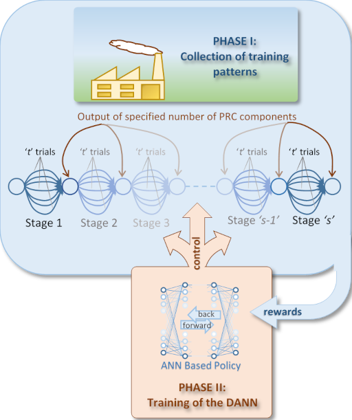
DANN development is a deeply nested process, as shown in Figure 5. The outer level of this process comprises two main phases: Phase I, the collection of training patterns through the exploration of alternative decision tracks; and, Phase II, the training of the DANN. These phases are cycled through a number of times until learning converges, each occasion using the most recent version of the DANN to control the simulation. Each time the system cycles back to Phase I, the simulation is reset to a new starting point. These phases are described in detail in the following two sections.
Collection of Training Patterns
Collecting training patterns is undertaken in a series of stages s, as illustrated in the upper blue section of Figure 5. Each stage experiments with a predefined number of trials t simulating the fabrication of a set of PRC components. The trial with the best production performance (see Section 4.1.1) is selected for later training of the DANN, and as the lead-in for the next stage in the simulation. The training patterns collected are the mappings from input to output for each state transition in the selected trial.
This process continues until a specified number of stages have been completed, each time collecting training patterns from the best performing trial. For future studies, parameters that can be investigated in terms of optimizing performance are the number of trials per stage, the number of PRC components to be fabricated per trial (this could be variable between stages), and the number of stages in the phase.
After completion of this phase, the system moves to DANN training before returning for another round of collecting training patterns. The intent is that by cycling between Phases I and II in this manner, the policy will move towards a better solution incrementally.
Delivery Performance
Delivery performance is measured in terms of delays to the delivery of PRC components, with smaller delays being more favorable. The cost function used for training is the root-mean-square (RMS) of these delays, as shown in Equation 1. Note, a PRC component could be delivered early (indicated by a negative delay) but the square operation would cancel the negative sign and thereby treat it as an equivalent delay. Therefore, the delays in this function are offset relative to a base value to give greater emphasis to actual delays over early deliveries.
where
is the delay for the PRC component at its completion;
is the number of PRC components completed at the current trial;
is the base value against which the delays are offset - this value is the maximum contingency time possible for a PRC component.
Rewards
The learning strategy presented here collects training patterns based on their success in improving system performance. For this reason, a training pattern's output values are modified from that produced by the DANN to increase the probability of making the same selection in a similar circumstance. The modification (a reward) is to move the selected output value closer to 1.0, and to move the other relevant output values closer to 0.0, remembering that the output values are treated as probabilities of selecting a RC component from the queue. The extent of the modification will be treated as an experimental hyper-parameter, although for this study the rewards are set to 0.0 and 1.0 without any discount.
DANN Training
The training patterns collected in Phase I are used to train the DANN, or to further train it in repeat cycles, as illustrated in the lower orange section of Figure 5.
The DANN was implemented in Python and PyTorch (Paszke et al., 2019), using the optimizer RMSProp (root-mean-square propagation) and the loss function MSELoss (mean-squared-error) with reduction set to mean. Data loading used a mini-batch size of 64 (with a training set size typically around 2,000 per cycle) with shuffling switched on. The learning rate was set to 0.001.
Training was conducted until the output from the loss function had converged, which was typically within 1,000 epochs. Testing of the system was undertaken after the RL learning cycle had plateaued. This involved running the simulation in implementation mode (see Section 3.3.3) using a start point not used for learning.
Results and Discussion
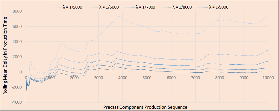
Ideally, there should be a balance between the demand for work (given by the batch size distribution for orders and their arrival rate, λ) and the factory's maximum output (determined in part by the handling times for the processes). An efficient control policy will allow this balance to be achieved in an optimal way, either by maximizing the amount of work taken-on without causing deliveries to be late, or minimize the number of productive resources needed to fulfill the demand. This study considers a situation where the demand is slightly in excess of the balance point, and then compares the performances of the alternative policy types (give in Section 3.2) to increase delivery performance (as measured in Section 4.1.1). The first experiment was performed to identify the arrival rate, λ, for orders that would give rise to this level of demand, given the handling times for the processes shown in Table 1. Figure 6 shows the results from running the factory simulation five times using a range of different order arrival rates (from to ). Each of these five simulations was run until a total of 10,000 individual PRC components were output (an average of 248 batches of PRC components per simulation run). Each curve shows the rolling average of the delays for the components across the 10,000 PRC component production runs. A rolling mean delay of 1,000, for example, indicates that on average the PRC components are delivered 1,000 time units late up to that point in the production run. The policy used to control the system was an untrained DANN. Based on these results, an order arrival rate of was selected as it appeared to create a demand that slightly exceeds the output from the factory. This is difficult to verify, however, due to the strong stochastic nature of the system's behavior. Future research should check the resilience of the DANN policy to changes in the order arrival rate.
A series of experiments were undertaken to assess the ability of the DANN to learn an efficient policy for controlling the PRC production process, to compare its performance with both the rule-of-thumb and random policies outlined in Section 3.2, and to test the sensitivity of its performance to varying the number of PRC components (N) that it evaluates at its input (see Section 3.3.1).
Learning Performance
The first performance experiment was designed to evaluate the ability of the DANN to learn using the proposed RL method described in Section 4. The parameters selected for the RL process were as follows:
- The number of cycles of Phases I and II was set to 20 (see Section 4.1, Figure 5) since initial experiments indicated that there was little learning being accumulated beyond this point.
- The maximum number of PRC components, N, to be evaluated in a queue by the DANN (see Section 3.3.1) was set to 20 since the queue lengths were rarely found to extend beyond this value for the system considered. Later, in Section 5.2, results are presented looking at the relationship between the value of N and performance.
- During Phase I in the training cycle, training data was collected over a 2,000 PRC component production run, divided into 100 stages of 20 PRC components each and with 100 trials per stage (see Section 4.1, Figure 5). Each cycle generated around 2,000 training patterns. Future work will investigate the relationship between these parameters and performance.
- Following the completion of each cycle, a testing run of the system was made for a sequence of 8,000 PRC components not used for training.
Figure 7 shows the performance of the DANN control policy over 20 cycles of the RL method. Performance is measured as the mean improvement in delivery time provided by the DANN (using the random policy as the benchmark, Section 3.2) over a simulated production run. The training runs were performed for a sequence of 2,000 PRC components (results shown in orange), while the testing runs were performed for a sequence of 8,000 PRC components (results shown in blue). Each point in the figure indicates the mean improvement at a given stage in the RL cycle. For example, the best performance for a training run occurred at the 3rd RL cycle, where the DANN policy (compared to the random policy) had a mean improvement in delivery time of 36.6 time units per PRC component.
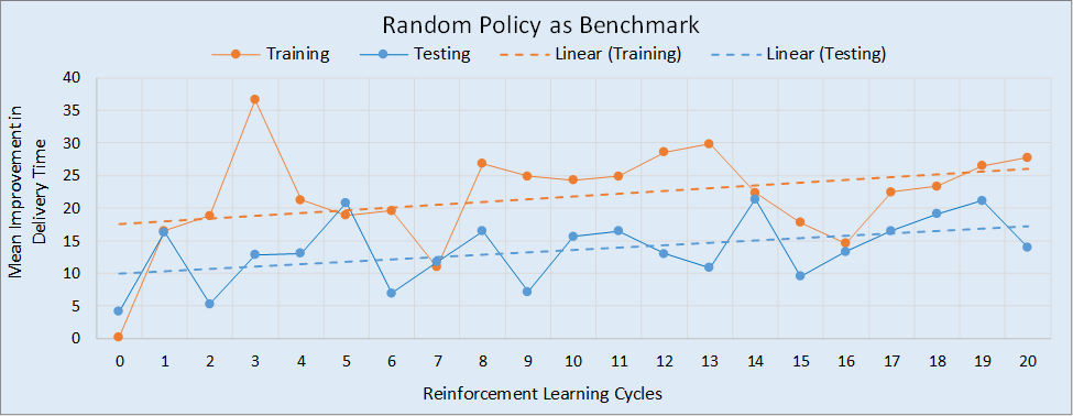
The best version of the DANN should be selected based on the testing run since it is independent of training and therefore does not have any potential inherent bias towards the trained DANN. Thus, for the 20 cycles considered, the best performing DANN was that generated at the 14th RL cycle, having a mean improvement in delivery time of 21.4 time units per PRC component (about 3.9% of the active processing time for an average PRC component). Clearly, in this regard, the DANN outperformed the random policy.
Figure 7 indicates that there is significant stochastic variance in the performance of the DANN over the RL cycles. For this reason, the linear trends for the two curves were also plotted on the figure. These trend lines indicate that both training and testing performance would likely improve if additional RL cycles were undertaken. The apparent positive trend for the testing performance suggests that the DANN is currently undertrained. The difference in the height of the two trend lines is to be expected, and is probably due to innate bias in the DANN to the data on which it was trained.
Figure 8 shows a similar plot to that of Figure 7, except that the performance of the DANN is measured using the rule-of-thumb policy as the benchmark rather than the random policy. The conclusions drawn from Figure 8 are similar to those from Figure 7, with the best version of the DANN being generated at the 14th RL cycle (according to the testing data), and with the DANN outperforming the rule-of-thumb policy, in this case by 23.2 time units per PRC component.
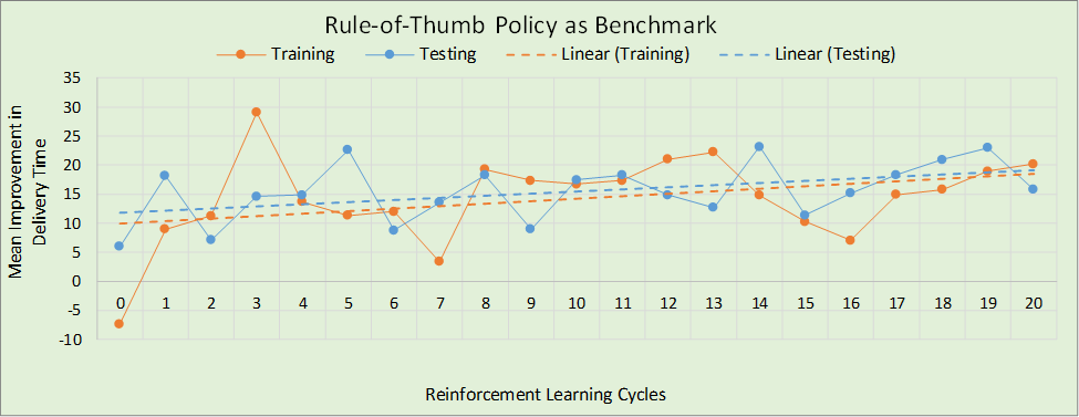
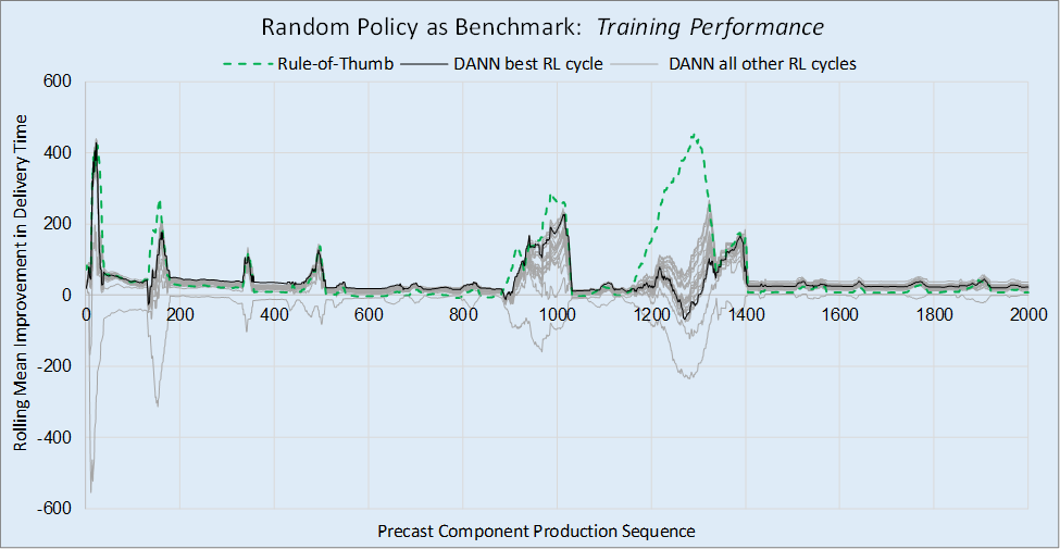
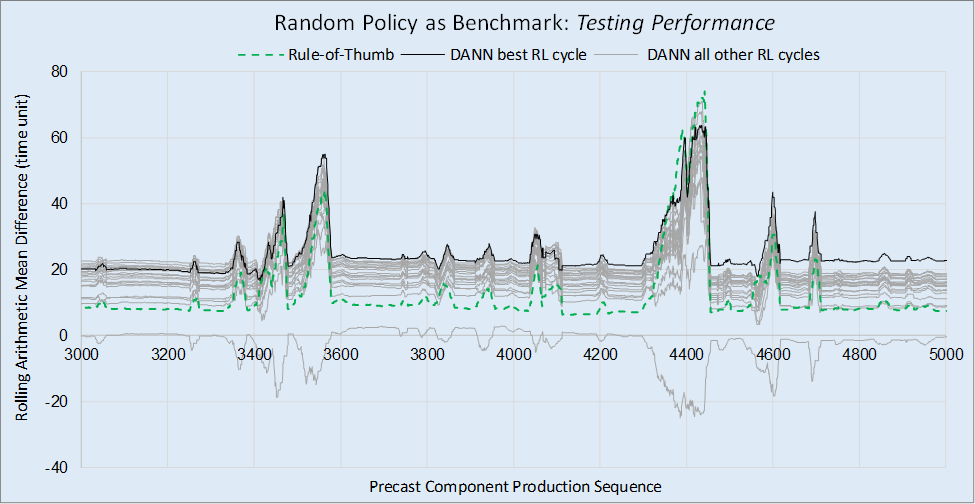
Figure 9 compares the performances of the rule-of-thumb policy and DANN policy at different RL cycles, using the random policy as the benchmark. The lines indicate the rolling mean improvement in delivery time, with the dashed green line representing the rule-of-thumb policy, the gray lines representing the DANN policy at various RL cycles, and the black line representing the best performing DANN policy. The lowest gray line in the figure represents the DANN policy before it underwent any training. The best performing DANN is that generated at RL cycle 14 as noted earlier.
Figure 9a shows the relative performances of the specified policies over the 2,000 training PRC component run. The most significant point on this graph is at the 2,000th PRC component as that indicates performance based on all the training data. Figure 9b shows the same but for 2,000 testing PRC components, taken from the middle of an 8,000 PRC component run. Looking at Figure 9b, it is clear that the best DANN policy significantly outperformed the rule-of thumb policy for most of the plot. However, around the 4,400 PRC components location, the rule-of-thumb policy accumulated large gains that briefly took it beyond the performance of the best DANN policy. Indeed, whenever the DANN policy and rule-of-thumb policies experienced large peaks in performance, it appears the rule-of-thumb policy improved more quickly. This suggests that more training of the DANN may be beneficial in the scenarios that lead to these peaks.
|
|
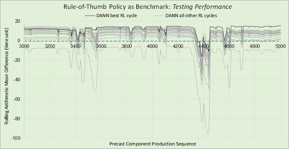
Figure 10 presents the same testing results as Figure 9b but with the DANN's performance benchmarked against the rule-of-thumb policy indicated by the dashed green line. This shows more clearly the relative performances of the DANN and rule-of-thumb policies. The best DANN policy tends to hover around a 14 to 15 time unit per PRC component advantage over the rule-of-thumb policy, but with occasion dips in relative performance.
Performance Dependence on the Number of PRC Components Sampled by the DANN
The experiments detailed in the previous section represent the initial formal training of the DANN, utilizing values for adjustable parameters selected based on the reasoning presented in Section 3.3.2 and Section 5.1. Future studies will be focused on optimizing the performance of the DANN by conducting a set of sensitivity analyses, exploring a comprehensive range of values for each DANN parameter including the number of hidden layers, the number of units per hidden layer, and the number of cycles of Phases I and II. As an example of how sensitivity analysis can be used to improve performance, this section considers optimizing the parameter N, the number of PRC components in a queue that can be evaluated for processing. As noted in Section 3.3.1, the input structure of a DANN is rigid and therefore the value for N has to be pre-determined. In the experiments reported above, N was set to a maximum of 20 PRC components. In this section, a sensitivity analysis is reported looking at the dependence of performance on the value of N, ranging from 5 to 30 in steps of 5 PRC components. These results are presented in Figure 11, with each curve representing the best DANN's generated over 20 RL training cycles for different values of N. Performance is shown for the last 2,000 PRC components in an 8,000 testing PRC component run, using the random policy as the benchmark. For comparison, the performance of the rule-of-thumb policy is also shown as a green dashed line. Note, the seed for the random number generators used in the stochastic sampling during simulation where different to the experiments in Section 5.1. This changed the absolute values generated in the production runs, but the characteristic performance behavior of the policies was similar.
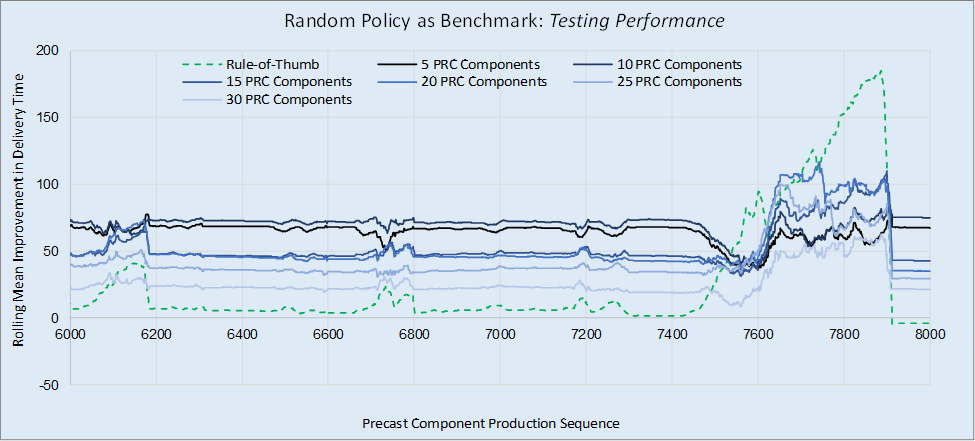
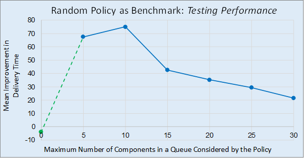
The optimum value for N was found to be 10 PRC components, providing a mean improvement in delivery time of 75.1. This is over twice the performance of the DANN trained with N set to the original value of 20, where the mean improvement in delivery time was found to be 35.3. A summary of the performances for the different values of N, measured at the end of the 8,000 testing PRC component run, is given in Figure 12. Note, the rule-of-thumb policy is equivalent to using a DANN with N set to 0, and is thus shown as such in this figure by the green marker. The overall form of the curve in Figure 12 is not surprising and can be explain as follows. The initial increase in performance (from N = 0 to 10) is likely due to an increase in the number of choices available to the DANN policy when selecting the next PRC component to start working. The subsequent decrease in performance (from N = 10 onwards) is possibly due to several reasons including the rapidly increasing sparsity of training patterns in higher dimensional input space. The constancy of this observation, and its dependence on other system attributes (such as work demand), requires further investigation. Future work will also consider developing an array of DANNs, each trained to serve queues of different lengths rather than a one-size-fits-all approach.
Conclusion and Future Work
The paper presented the development and evaluation of a DANN-based policy for controlling a construction factory producing PRC components, trained using RL techniques. Control was concerned with selecting PRC components from a queue for processing (when the process became available) with the aim of optimizing delivery performance. The performance of the DANN policy was compared to a rule-of-thumb and a random selection policy. The DANN was developed and tested using a simulation of an actual precast reinforced concrete factory.
A primary goal of this study was to determine if the DANN approach could cope with the unique challenges posed by the construction industry. The DANN proved able to learn an effective and reliable policy operating within this environment, and was found to significantly outperform the rule-of-thumb and random policies over long production runs (of 8,000 PRC components) except on some rare occasions.
An analysis of the progress of learning during the RL procedure indicated that addition training cycles, beyond the 20 considered, would likely improve the performance of the DANN policy. Furthermore, performance was found to be strongly dependent on the value adopted for N (the maximum number of PRC components in a queue considered for processing by the DANN). Based on these analyses, it is clear that the performance of the DANN has potential for further improvement. Indeed, there are many other parameters open to experiment that could further optimize performance, including:
- Undertaking sensitivity analyses on the structure and architecture of the DANN, including experimenting with the number of hidden layers, the number of hidden units per layer, and the inclusion of an ensemble of models.
- Increasing the length and diversity of production runs used for training, thereby increasing the size and scope of the training dataset.
- Undertaking sensitivity analyses on the RL hyper-parameters such as the reward term lengths, the rewards discount rate, the number of trials per stage, and the number of stages in a cycle.
- Testing the performance of alternative RL algorithms.
The following work is planned to increase the scope of application of the approach:
- Case studies aimed at identifying detailed performance data, logistics, and the practical issues associated with day-to-day control of construction manufacturing systems. This would include the use of alternative cost functions that reflect the range of objectives that different manufactures may consider important.
- Increasing the range of state data used for input and the scope of the type of decisions made by the decision agent.
Finally, a study is proposed comparing the performance of the RL-based DANN approach with heuristic search techniques to solve the same class of problems, considering both delivery performance and decision processing time.
Bibliography
- Benjaoran, V. & Dawood, N. (2005). An Application of Artificial Intelligence Planner for Bespoke Precast Concrete Production Planning: A Case Study.

- Chan, W. T. & Hu, H. (2002). Production Scheduling for Precast Plants Using a Flow Shop Sequencing Model. Journal of Computing in Civil Engineering, 16(3), 165-174.

- Flood, I. (1989). A Neural Network Approach to the Sequencing of Construction Tasks. In Proceedings of the 6th International Symposium on Automation and Robotics in Construction (pp. 204-211). San Francisco, CA: IAARC.

- Flood, I. & Flood, P. D. L. (2022). Intelligent Control of Construction Manufacturing Processes Using Deep Reinforcement Learning. In Proceedings of the 12th International Conference on Simulation and Modeling Methodologies, Technologies and Applications (SIMULTECH 2022) (pp. 112-122). Lisbon, Portugal: SCITEPRESS.


- Glorot, X., Bordes, A., & Bengio, Y. (2011). Deep Sparse Rectifier Neural Networks. In Proceedings of the Fourteenth International Conference on Artificial Intelligence and Statistics (pp. 315-323). Proceedings of Machine Learning Research, vol 15. Fort Lauderdale, FL: PMLR.


- Iba, H. & Noman, N. (Eds.) (2020). Deep Neural Evolution: Deep Learning with Evolutionary Computation. Natural Computing Series, Springer Singapore.

- Leu, S. & Hwang, S. (2001). Optimal Repetitive Scheduling Model with Shareble Resource Constraint. Journal of Construction Engineering and Management, 127(4), 270-280.

- Paszke, A., Gross, S., Massa, F., Lerer, A., Bradbury, J., Chanan, G., Killen, T., Lin, Z., Gimelshein, N., Antiga, L., Desmaison, A., Köpf, A., Yang, E., DeVito, Z., Raison, M., Tejani, A., Chilamkurthy, S., Steiner, B., Fang, L., Bai, J., & Chintala, S. (2019). PyTorch: An Imperative Style, High-Performance Deep Learning Library. In Wallach, H., Larochelle, H., Beygelzimer, A., d'Alché-Buc, F., Fox, E., & Garnett, R. (eds) Advances in Neural Information Processing Systems 32 (pp. 8024–8035). Red Hook, NY: Curran Associates, Inc.

- Shitole, V., Louis, J., & Tadepalli, P. (2019). Optimizing Earth Moving Operations via Reinforcement Learning, In Proceedings of the 2019 Winter Simulation Conference (pp. 2954-2965). Piscataway, NJ: IEEE

- Sutton, R. & Barto, A. (2018). Reinforcement Learning: An Introduction (2nd ed.). Cambridge, MA: The MIT Press.
- Wang, Z., Hu, H., & Gong. J. (2018). Framework for Modeling Operational Uncertainty to Optimize Offsite Production Scheduling of Precast Components. Automation in Construction, 86, 69-80.

- Waschneck, B., Reichstaller, A., Belzner, L., Altenmüller, T., Bauernhansl, T., Knapp, A., & Kyek, A. (2018). Optimization of Global Production Scheduling with Deep Reinforcement Learning. Procedia CIRP, 72, 1264-1269.

- Xia, K., Sacco, C., Kirkpatrick, M., Saidy, C., Nguyen, L., Kircaliali, A., & Harik, R. (2021). A Digital Twin to Train Deep Reinforcement Learning Agent for Smart Manufacturing Plants: Environment, Interfaces and Intelligence. Journal of Manufacturing Systems, 58 Part B, 210-230.

- Zhou, L., Zhang, L., & Horn, B. K. P. (2020). Deep Reinforcement Learning-Based Dynamic Scheduling in Smart Manufacturing. Procedia CIRP, 93, 383-388.

Copyright Information
 Copyright © 2023 Ian Flood, Xiaoyan Zhou. This article is licensed under a Creative Commons Attribution 4.0 International
License.
 Journal of
Simulation Engineering, Volume 3 (2022/2023). Article URL: https://articles.jsime.org/3/2