
Simulation Framework for Asynchronous Iterative Methods
ACM Subject Categories
Hardware~Fault toleranceComputing methodologies~Linear algebra algorithmsApplied computing~Mathematics and statistics
Keywords
- Asynchronous Iterative Methods
- Fault Tolerance
- Asynchronous Simulation
- Shared Memory
- Intel® Xeon Phi™
Abstract
As high-performance computing (HPC) platforms progress towards exascale, computational methods must be revamped to successfully leverage them. In particular, (1) asynchronous methods become of great importance because synchronization becomes prohibitively expensive and (2) resilience of computations must be achieved, e.g., using checkpointing selectively which may otherwise become prohibitively expensive due to the sheer scale of the computing environment. In this work, a simulation framework for asynchronous iterative methods is proposed and tested on HPC accelerator (shared-memory) architecture. The design proposed here offers a lightweight alternative to existing computational frameworks to allow for easy experimentation with various relaxation iterative techniques, solution updating schemes, and predicted performance. The simulation framework is implemented in MATLAB® using function handles, which offers a modular and easily extensible design. An example of a case study using the simulation framework is presented to examine the efficacy of different checkpointing schemes for asynchronous relaxation methods.
Introduction
Asynchronous iterative methods are increasing in popularity recently due to their ability to be parallelized naturally on modern co-processors such as GPUs and Intel® Xeon Phi™. Many examples of recent work using fine-grained parallel methods are available (see Anzt, Dongarra, & Quintana-Ortí, 2016, Anzt, 2012, Chow, Anzt, & Dongarra, 2015, Chow & Patel, 2015, Anzt, Chow, & Dongarra, 2015 and many others in Section 2). A specific area of interest is on techniques that utilize fixed point iteration, i.e., those techniques that solve equations of the form
for some vector 𝑥 ∈ 𝐷 and some map 𝐺 : 𝐷 → 𝐷. These techniques are well suited for fine-grained computation and they can be executed either synchronously or asynchronously, which helps tolerate latency in high-performance computing (HPC) environments. Looking forward to the future of HPC, it is important to prioritize the develop of algorithms that are resilient to faults since on future platforms, the rate at which faults occur is expected to increase dramatically (Cappello et al., 2009; Cappello et al., 2014; Asanović et al., 2006; Geist & Lucas, 2009).
While many asynchronous methods are designed for shared memory architectures and asynchronous iterative methods have gained popularity for their efficient use of resources on shared memory accelerators in modern HPC environments (Venkatasubramanian & Vuduc, 2009), lately there has been some work done at improving the performance of asynchronous iterative methods in distributed memory environments. Such works include attempts to implement asynchronous iterative methods in MPI-3 using one sided remote memory access (Gerstenberger, Besta, & Hoefler, 2014) as well as efforts to reduce the cost of communication in these environments (Wolfson-Pou & Chow, 2016).
Developing algorithms that are resilient to faults is of paramount importance, and fine-grained parallel fixed point methods are no exception. In this paper, we propose a simulation framework that can help developing algorithms resilient to faults. These types of frameworks allow for experimentation that is not specific to any singular platform or hardware architectures and allows experiments to simulate performance on both current computing environments and look at how those results may continue to evolve along with the computer hardware. Hence, they enable the possibility to: (1) test and validate different fault-models (which are still emerging), (2) experiment with different checkpointing libraries/mechanisms, and (3) help in efficiently implementing asynchronous iterative methods. Additionally, it can be difficult to implement asynchronous iterative methods on a variety of architectures to observe performance behavior in different computing environments, and having a working simulation framework allows users to conduct extensive experiments without any major programming investment.
This study aims to develop a simulation framework that is focused on the performance of asynchronous iterative methods. The goal is to produce a lightweight computational framework capable of being used for various asynchronous iterative methods, with an emphasis on methods for solving linear systems, and simulating the performance of these methods on shared memory devices. The contributions of this work are
- the development, testing, and validation of a modular simulation framework for asynchronous iterative methods that can be used in the creation of new and improved algorithms,
- a process for the generation of time models from HPC implementation code, which may be used to initialize the framework,
- a case study on how to use the framework in the development of fault tolerant algorithms, and
- a comparison of several implementations of an asynchronous iterative relaxation method, used in the proposed framework.
The simulation framework developed here is capable of predicting performance on various HPC system configurations and to show the performance of an algorithm subject to resiliency or reproducibility requirements.
The rest of this paper is organized as follows. Section 2 provides a brief summary of related studies. Section 3 gives an overview of asynchronous iterative methods, while Section 4 describes the design and utilization of the simulation framework in modeling the behavior of these methods. Section 5 describes a process for collecting time data from HPC implementations and developing time models from the data for use in the simulation framework. A comparison of different implementations is given in Section 5.3, while framework validation is considered in Section 5.4. Section 6 gives background information related to the creation of efficient checkpointing routines and provides a series of numerical results. Section 7 provides conclusions.
Related Work
Development of computational frameworks for the purposes of simulating performance has a long history in the literature. Examples of such frameworks include SimGrid (Casanova, 2001; Casanova, Legrand, & Quinson, 2008) that focuses on distributed experiments, GangSim (Dumitrescu & Foster, 2005) and GridSim (Buyya & Murshed, 2002) that focus on grid scheduling, and CloudSim (Calheiros, Ranjan, De Rose, & Buyya, 2009; Calheiros, Ranjan, Beloglazov, De Rose, & Buyya, 2011) that models performance of cloud computing environments. These environments focus on specific HPC implementation features, such as job scheduling and data movement, and on providing a view of how the systems themselves behave in HPC-like scenarios. On the other hand, the framework developed here is intended to simulate not only the HPC performance but also the algorithmic performance of a particular class of problems (e.g., iterative convergence to a linear system solution) under various system configurations (e.g., asynchronous thread behavior in shared-memory systems) and with various additional requirements (e.g., resiliency or reproducibility).
The class of problems that the framework proposed in this study addresses are stationary solvers, also referred to as relaxation methods. The focus is on the behavior of these methods in asynchronous computing environments. However, the framework also easily admits synchronous updates; the key is the fine-grained nature of the algorithm. Fine-grained parallel methods, specifically parallel fixed point methods, are an area of increased research activity due to their practical use on HPC environments. An initial exploration of fault tolerance for stationary iterative linear solvers (i.e., Jacobi) is given in (Anzt, Dongarra, & Quintana-Ortí, 2015) and expanded on (Anzt, Dongarra, & Quintana-Ortí, 2016). The general convergence of parallel fixed point methods has been explored extensively (Addou & Benahmed, 2005; Frommer & Szyld, 2000; Bertsekas & Tsitsiklis, 1989; Ortega & Rheinboldt, 2000; Baudet, 1978; Benahmed, 2007).
Examples of work examining the performance of asynchronous iterative methods include an in-depth analysis from the perspective of utilizing a system with a co-processor (Anzt, 2012; Avron, Druinsky, & Gupta, 2015), as well as performance analysis of asynchronous methods (Bethune, Bull, Dingle, & Higham, 2011; Bethune, Bull, Dingle, & Higham, 2014; Hook, & Dingle, 2018). In particular, both (Bethune, Bull, Dingle, & Higham, 2011) and (Bethune, Bull, Dingle, & Higham, 2014) focus on low level analysis of the asynchronous Jacobi method, similar to the example problem that is featured here. While many recent research results for asynchronous iterative methods are focused on implementations that utilize a shared memory architecture, one area of asynchronous iterative methods that has seen significant development using a distributed memory architecture is optimization (Cheung & Cole, 2016; Iutzeler, Bianchi, Ciblat, & Hachem, 2013; Hong, 2017; Zhong & Cassandras, 2010; Srivastava & Cassandras, 2011; Tsitsiklis, Bertsekas, & Athans, 1986; Boyd, Parikh, Chu, Peleato, & Eckstein, 2011).
The use case of the simulation framework that is featured in Section 6 shows the ability of the framework to be used in the development of fault tolerance techniques. The development of these techniques is important as HPC platforms continue to become both larger and more susceptible to faults. The expected increase in faults for future HPC systems is detailed in a variety of different sources. A high level article detailing the expected increase in failure rate from a reasonably non-technical point of view is available in the various versions of the "Monster in the Closet" talk and paper (Geist, 2011; Geist, 2012; Geist, 2016). More technical and detailed reports are given in a variety of sources composed of groups of different researchers from both academia and industry (Asanović et al., 2006; Cappello et al., 2009; Cappello et al., 2014; Snir et al., 2014; Geist & Lucas, 2009). Additionally, the Department of Energy has commissioned two very detailed reports about the progression towards exascale level computing; one from a general computing standpoint (Ashby et al., 2010), and a report aimed specifically at applied mathematics for exascale computing (Dongarra et al., 2014). Fault tolerance for fine-grained asynchronous iterative methods has been studied at a fundamental level (Gärtner, 1999; Coleman & Sosonkina, 2017), as well as made specific to certain algorithms (Coleman, Sosonkina, & Chow, 2017; Coleman, & Sosonkina, 2018; Anzt, Dongarra, & Quintana-Ortí, 2015; Anzt, Dongarra, & Quintana-Ortí, 2016). Fault tolerance for synchronous fixed point algorithms from a numerical analysis has been investigated in (Stoyanov & Webster, 2015). Error correction for GPU based oriented asynchronous methods were investigated in (Anzt, Luszczek, Dongarra, & Heuveline, 2012).
Several numerically based fault models similar to the one that is used in this study have been developed recently, and are used as a basis for the generalized fault simulation that is developed here. These include a "numerical" fault model that is predicated on shuffling the components of an important data structure (Elliott, Hoemmen, & Mueller, 2015), and a perturbation based model put forth in (Stoyanov & Webster, 2015) and (Coleman & Sosonkina, 2016b). Other models that are not based upon directly injecting a bit flip, such as inducing a small shift to a single component of a vector have been considered as well (Hoemmen & Heroux, 2011; Bridges, Ferreira, Heroux, & Hoemmen, 2012). Comparisons between various numerical soft fault models have been made in (Coleman & Sosonkina, 2016a; Coleman, Jamal, Baboulin, Khabou, & Sosonkina, 2018).
Asynchronous Iterative Methods
In fine-grained parallel computation, each component of the problem (i.e., a matrix or vector entry) is updated in a manner that does not require information from the computations involving other components while the update is being made. This allows for each computing element (e.g., for a single processor, CUDA core, or Xeon Phi™ core) to act independently from all other computing elements. Depending on the size of both the problem and the computing environment, each computing element may be responsible for updating a single entry to update, or may be assigned a block that contains multiple components. The generalized mathematical model that is used throughout this paper comes from (Frommer & Szyld, 2000), which in turn comes from (Chazan & Miranker, 1969; Baudet, 1978; Szyld, 1998) among many others.
To keep the mathematical model as general as possible, consider a function, 𝐺 : 𝐷 → 𝐷, where 𝐷 is a domain that represents a product space 𝐷 = 𝐷1 × 𝐷2 × … × 𝐷2. The goal is to find a fixed point of the function 𝐺 inside of the domain 𝐷. To this end, a fixed point iteration is performed, such that
and a fixed point is declared if 𝑥𝑘+1 ≈ 𝑥𝑘. Note that the function 𝐺 has internal component functions 𝐺𝑖 for each sub-domain, 𝐷𝑖, in the product space, 𝐷. In particular, 𝐺𝑖 : 𝐷 → 𝐷𝑖, which gives that
As a concrete example, let each 𝐷𝑖 = ℝ . Forming the product space of each of these 𝐷𝑖's gives that 𝐷 = ℝ𝑚 . This leads to the more formal functional mapping, 𝑓 : ℝ𝑚 → ℝ𝑚 . Additionally, let . In this case, each of the individual 𝑓𝑖 component functions is defined by . Note that each component functions operates on all of the vector even if the individual function definition does not require all of the components of to perform its specific update.
The assumption is also made that there is some finite number of processing elements 𝑃1, 𝑃2, …, 𝑃𝑝 each of which is assigned to a block 𝐵 of components 𝐵1, 𝐵2, …, 𝐵𝑚 to update. Note that the number 𝑝 of processing elements will typically be significantly smaller than the number 𝑚 of blocks to update. With these assumptions, the computational model can be stated in Algorithm 1.
Algorithm 1 General computational model
1:for each processing element do
2:for until convergence do
3:Read from common memory
4:Compute for all
5:Update in common memory with for all
6:end for
7:end for
This computational model has each processing element read all pertinent data from global memory that is accessible by each of the processors, update the pieces of data specific to the component functions that it has been assigned, and update those components in the global memory. Note that the computational model presented in Algorithm 1 allows for either synchronous or asynchronous computation; it only prescribes that an update has to be made as an "atomic" operation (in line 5), i.e., without interleaving of its result. If each processing element 𝑃𝑙 is to wait for the other processors to finish each update, then the model describes a parallel synchronous form of computation. On the other hand, if no order is established for 𝑃𝑙s, then an asynchronous form of computation arises.
To continue formalizing this computational model a few more definitions are necessary. First, set a global iteration counter 𝑘 that increases every time any processor reads from common memory. At the end of the work done by any individual processor, 𝑝, the components associated with the block 𝐵𝑝 will be updated. This results in a vector, where the function 𝑠𝑙(𝑘) indicates how many times an specific component has been updated. Finally, a set of individual components can be grouped into a set, 𝐼𝑘 , that contains all of the components that were updated on the 𝑘th iteration. Given these basic definitions, the three following conditions (along with the model presented in Algorithm 1) provide a working mathematical framework for fine-grained asynchronous computation.
Definition 1. If the following three conditions hold
- , i.e., only components that have finished computing are used in the current approximation.
- , i.e., the newest updates for each component are used.
- , i.e., all components will continue to be updated.
Then given an initial , the iterative update process defined by
where the function uses the latest updates available is called an asynchronous iteration.
This basic computational model (i.e., the combination of Algorithm 1 and Definition 1 together) allows for many different results on fine-grained iterative methods that are both synchronous and asynchronous, though the three conditions given in Definition 1 are unnecessary in the synchronous case.
Asynchronous Relaxation Methods
Relaxation methods have been the focus of many of the works mentioned in Section 2 such as (Chazan & Miranker, 1969) and (Baudet, 1978); a much more detailed description can be found in (Bertsekas & Tsitsiklis, 1989) among many other sources. This section provides an introduction that will serve as a reference for the later work in this study.
Relaxation methods can be expressed as general fixed point iterations of the form
where 𝐶 is the 𝑛 × 𝑛 iteration matrix, 𝑥 is an 𝑥-dimensional vector that represents the solution, and 𝑑 is another 𝑥-dimensional vector that can be used to help define the particular problem at hand.
The Jacobi method is an asynchronous relaxation method built for solving linear systems of the form
and following the methodology put forth in (Bertsekas & Tsitsiklis, 1989), this can be broken down to view a specific row — say the 𝑖th — of the matrix 𝐴,
and this equation can be solved for the 𝑖th component of the solution, 𝑥𝑖, to give,
This equation can then be computed in an iterative manner in order to give successive updates to the solution vector. In synchronous computing environments, each update to an element of the solution vector, 𝑥𝑖 is computed sequentially using the same data for the other components of the solution vector (i.e., the 𝑥𝑗, in Equation (2). Conversely, in an asynchronous computing environment, each update to an element of the solution vector occurs when the computing element responsible for updating that component is ready to write the update to memory and the other components used are simply the latest ones available to the computing element.
Expressing Equation (2) in a block matrix form more similar to the original form of the iteration expressed in Equation (1),
where 𝐷 is the diagonal portion of 𝐴, and 𝐿 and 𝑈 are the strictly lower and upper triangular portions of 𝐴 respectively. This gives an iteration matrix of 𝐶 = -𝐷−1(𝐿 + 𝑈) .
Convergence of asynchronous fixed point methods of the form presented in Equation (1) is determined by the spectral radius of the iteration matrix, 𝐶, and dates back to the pioneering work done by both (Chazan & Miranker, 1969) and (Baudet, 1978):
Theorem 1. For a fixed point iteration of the form given in Equation (1) that adheres to the asynchronous computational model provided by Algorithm 1 and Definition 1, if the spectral radius of 𝐶, ρ(|𝐶|), is less than one, then the iterative method will converge to the fixed point solution.
As noted in (Wolfson-Pou & Chow, 2016), the iteration matrix 𝐶 that is used in the Jacobi relaxation method serves as a worst case for relaxation methods of the form discussed here. However, because of the ubiquitous use of the Jacobi method in parallel solutions of large problems in many different domains in science and engineering we use the Asynchronous (Block) Jacobi method predominantly throughout the remainder of this study. Note that many of the concepts and ideas expressed in this paper can be easily adapted to more complex algorithms.
Design of Simulation Framework
The simulation framework proposed here is designed to simulate the performance of an asynchronous iterative method operating on multiple computing elements using a single processing element. In this simulation framework, the emphasis is on fixed-point iterations1
for some . In the framework, certain components are assigned (possibly distinct) times for performing an update to their components, and the effects of various delay structures can be examined.
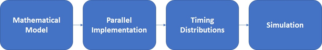
The development of the present computational framework is shown by the flow diagram in Figure 1, which is typical for computation frameworks, except for the third Timing Distributions stage. A mathematical formulation of a problem (e.g., as a set of equations) is presented first (Mathematical Model stage). The mathematical model is then implemented in an HPC environment (Parallel Implementation stage). Timing and algorithm-performance data (e.g., iterations to convergence) are collected from parallel executions on a subset of configurations and problem sizes, such that, in the proposed framework, timing distributions may be constructed (Timing Distributions stage) and used to simulate the performance of the mathematical model for target configurations and requirements. Since such simulations are faster and less-cumbersome to set-up, they allow for easy experimenting with variations of the underlying mathematical model, parallel implementation type and environment, or, eventually, in the expected performance.
The simulation framework developed here works to simulate the performance of generic asynchronous relaxation methods in shared memory environments. The simulation framework can then be modified to reflect changes in the environment, or else can be utilized to demonstrate the effectiveness of algorithmic modifications.
As a simple example, take 𝑛 = 2. Then and, using the terminology of Section 3,
In a traditional fully synchronous environment, both functions, 𝐺1 and 𝐺2, would be called simultaneously and no subsequent calls would be executed until both functions had returned and synchronized all results. In a fully asynchronous environment, both functions would be allowed to execute again immediately upon their own return, leading to a case where one of 𝑥1 or 𝑥2 may be updated more frequently than the other. Per Definition 1, both functions use the latest values of that are available to them when the function call is initiated. For instance, if the processing element that was assigned to update the component 𝑥1 was ten times as fast as the processing element assigned to update 𝑥2, then in the amount of time needed to update 𝑥2 once, the component 𝑥1 will have been updated ten times, and when 𝐺2 is called for the second time it will be called using the latest component of 𝑥1 (which has been updated 10 times), and the latest component of 𝑥2 (which has only been updated once).
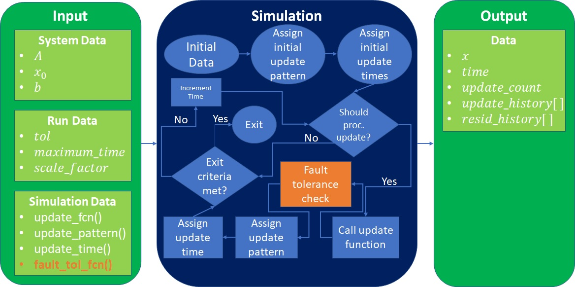
A block diagram showing the flow of the simulation framework is provided in Figure 2. The framework models the performance of methods that solve the linear system
using relaxation methods in either a synchronous or asynchronous manner.
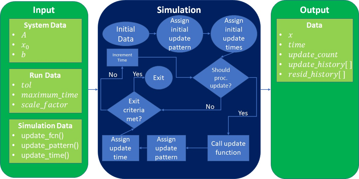
The simulation requires as input the matrix 𝐴, the right hand side 𝑏 and an initial guess at the solution, 𝑥0. The important pieces of the simulation are all passed as functions to the tool. There are three functions required:
- An update function that specifies how to perform the relaxation. A common technique for this is given by Equation (2). It is certainly possible to modify this equation to obtain different updates, as described, e.g., in (Saad, 2003).
- An update pattern function that determines which elements of the matrix 𝐴 are assigned to each simulated processor. A common technique for this assignment, is to evenly divide the work among all of the available processors, however other patterns are also possible. For example, the use of randomization in the solution of linear systems via relaxation methods has gained some popularity in the fields of optimization and machine learning (see, e.g., (Avron, Druinsky, & Gupta, 2015) and references therein) and update patterns such as this are easy to implement inside of this framework.
- An update time function that captures the empirical information that was captured from parallel performance runs on the HPC hardware. This function will typically be used to sample from the timing distribution that was generated beforehand. Note that, since each simulated processor makes calls to this function independently, the simulated performance will be asynchronous so long as the function returns different values upon different calls. Defining an update time function that has constant return (or constant return for every processor) provides a means to show synchronous performance.
By varying the three functions that are passed to the framework, not only can the HPC performance be predicted by making changes to the update time function, but various modifications to the basic algorithm can be quickly and easily compared in a manner that reflects real world asynchronous performance. With the renewed research interest in asynchronous iterative methods that perform relaxation updates, oftentimes performance between new variants and existing algorithms is only compared in simple synchronous experiments; the simulation framework proposed here allows for a more meaningful comparison between methods that does not require development of parallel implementations of all the methods or algorithm variations that are involved.
The simulation framework requires some data that specifies parameters concerning the particular run of the simulation such as the desired tolerance, the number of processors to simulate, and a computational scale factor. The framework itself is developed in MATLAB® and the three required functions are passed as function handles.
The simulation itself (see Simulation block in Figure 2) progresses by reading in the user provided input data, assigning an initial update pattern and time to each processor, and then beginning the main loop. Inside of the main loop, the time increments and a check is performed to see if the current time matches with the scheduled update time for any of the processors, if so, the update function is called and then a time for the next update is assigned to the processor that just updated and (if desired) the update pattern for the current processor is changed. After this, a check is performed on the size of the residual to determine if the exit criteria is met before the time is incremented again and the loop starts over. A pseudocode representation of the simulation framework for simulated asynchronous Jacobi is given in Algorithm 2.
Algorithm 2 Asynchronous Jacobi simulation
1:Input: , initial guess for , a number of processing elements , an input random number distribution
2:Output: Solution vector
3:Assign processor update times. by sampling from an appropriate random number distribution
4:Assign elements to each simulated processing element
5:for until convergence do
6:for each processing element do
7:if then
8:for each element assigned to do
9:
10:end for
11:Retrieve a new update time by sampling from the input distribution
12:end if
13:end for
14:Calculate the residual as in Equation (3) and check termination conditions
15:end for
Algorithm 2, a given update time τ𝑙 will often not be sampled as an integer. The simulation adjusts for this by scaling the number that is sampled by the appropriate order of magnitude, adjusting the maximum value allowed for 𝑡 accordingly, and then scaling back the final time calculated by the simulation. For example, if the desired time precision is hundredths of a second, and the time resulting for the first sampling of τ𝑙 was 1.234𝑠, then the simulation would perform the following steps:
where 𝑠 referenced is the scale_factor
defined in the block diagram given by Figure 2. For
example, if the desired precision is hundredths of a second, 𝑠 = 102, and the sampled value τ𝑙 becomes
Inside of the simulation framework, time is abstracted away to units
of time
, and then the final time is scaled back into the appropriate
units. This allows the framework to be adapted to future HPC environments,
as well as examining the impact of the standard variance of single core
performance on multi-core hardware elements if the method that is used is
tuned to be completely asynchronous. It should be possible — by adding or
removing appropriate communication penalties — to simulate the performance
of different memory architectures (e.g., distributed or cloud computing
environments). This is left as future work although the method for doing
this inside of the proposed framework is straightforward.
Sample Use-Cases for the Framework
Let the matrix 𝐴 result from a simple two dimensional finite-difference discretization of the Laplacian over a 10 × 10 grid, resulting in a 100 × 100 matrix with an average of 4.6 non-zero entries per row. The Laplacian
is a partial differential equation (PDE) commonly found in both science and engineering. The example problems taken in this study can be thought of as simulating the diffusion of heat across a two dimensional surface given some heat source along the boundary of the problem.
Once the PDE is discretized over the desired grid using finite differences, typically central finite differences, the linear system
is set up to be solved for a random right-hand side b that represents the desired boundary conditions. All problems considered in this study use Dirichlet boundary conditions. For the examples in this particular subsection, the righthand side is generated by taking each component sampled as a uniform random number between −0:5 and 0:5, and then normalizing the resultant vector. The iterative Jacobi method proceeds until the residual
is reduced past some desired threshold.
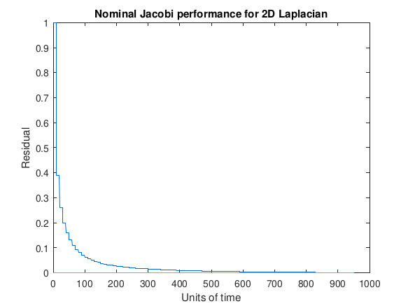
To begin with, an example of nominal performance of the solution of the two dimensional Laplacian in a synchronous environment is provided by Figure 3.
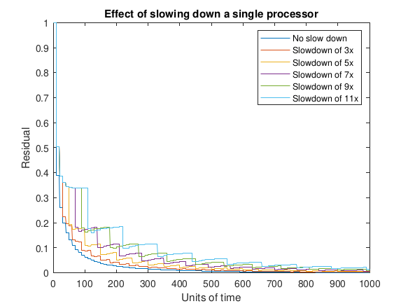
Next, consider the same problem from above, but in two slightly more complicated scenarios. In Figure 4 one of the ten processors involved in updating blocks of components of 𝑥 is provided updates more slowly than the other processors. This could reflect the scenario where updates are either performed synchronously or asynchronously where the effect of variance in performance is negligible, and a single processor has degraded performance. This can also be viewed as a look at the impact of asynchronous behavior on the Jacobi algorithm. Each curve shows the progression of the (global) residual subject to having a single slower processor with different degrees of slowdown (from zero to 11x).
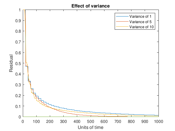
In Figure 5 the processor updates are not restricted to occur synchronously. Instead, the processors are assumed to have similar performance and perform their updates in time 𝑡𝑖 ∼ 𝑁(u, σ2) where the mean is set to 10 units of time and the variance is different for each curve depicted in the plot. An increase in the variance of processor performance, regardless of the timing distribution, could come about for a variety of reasons; an example of a scenario in the future could be having chips with more cores and lower voltage that are designed to address the challenges in creating very large scale HPC environments.
Asynchronous Jacobi Implementations for the Framework
Figure 4 and Figure 5 show relative differences in compute times among sharedmemory computing elements for a specific problem and a specific asynchronous iterative method. A more general simulation framework, which can be used for modeling and testing any synchronous or asynchronous iterative relaxation method, is presented here. Baseline, non-resilient method behavior may be reproduced in the framework; further, the user may also investigate fault injection and checkpointing.
The user decomposes the method according to the input parameters required
by the simulation framework. The update function that performs the
relaxation has an associated operational time, both of which are defined
by the user. Functionality within the relaxation may be isolated into
discrete operations with corresponding time information; the level of
granularity is decided by the user. For example, time to complete an
operation in the simulation framework may be modeled with a probability
density function derived from empirical data. To model time to perform
specific operations or calculations during method execution, data is
collected from the application during execution. In the implementation
code, operations are enclosed within calls to time functions, which
measure time to perform the operations. In this work the OpenMP®
library function
omp_get_wtime()
is used to measure wall time. For HPC implementations that use MPI,
MPI_Wtime()
may be used to measure wall time. Fine-grained operations in the code
should not overlap such that measurements overlap, i.e., for one
operation, do not measure time function calls of another operation. After
taking sufficient measurements, an operation is modeled by fitting a
probability density function to a normalized histogram of the time data.
This function may be included as part of the input to the framework. Note
that when comparing simulated run times with HPC run times, it may be
preferable to use an unmodified version of the HPC implementation code
that does not have time function calls and mechanisms for storing or
printing times. These functions and activities may increase run time and
provide an inaccurate metric for comparison.
This section describes two asynchronous relaxation method implementations and two corresponding use cases of the simulation framework. For both implementations, the test problem is a two dimensional discretization of the Laplacian
where the right-hand side is initialized with Dirichlet boundary conditions. Both implementations use OpenMP® for shared-memory parallelism and are executed on the shared-memory computing platform nicknamed Rulfo, which is an Intel® Xeon Phi™ Knight's Landing2 having 7210 model processor with 64 cores. Each core may optimally execute 4 threads for 256 threads total, and runs at 1.30 GHz. The simulation framework and experiments were implemented in MATLAB® R2018a, while the Jacobi implementations were written in C/C++ using the Intel C compiler version 17.04 and OpenMP® version 4.5.
Implementation 1: General Jacobi Solver
In this case, the heat problem is represented mathematically by a sparse matrix, which is solved by an asynchronous general Jacobi method. The Laplacian is generated over a 100 × 100 grid resulting in a matrix of size 10,000 × 10,000 with 49,600 non-zeros with an average of 4.96 non-zeros per row. The vector b from the resulting linear system,
is initialized such that the final solution vector has 𝑥𝑖 = 1 for all 𝑖. The initial guess 𝑥0 is all zeros.
In this implementation, all threads but one perform relaxations on assigned components, and a dedicated thread computes the global residual norm value 𝑏−𝐴𝑥(𝑡) that determines satisfactory convergence. Each thread retrieves the data it needs from shared memory, performs the necessary computations, and, in the case of the relaxation threads, writes the result back to shared memory. Synchronous shared-memory implementations of all classes of algorithms commonly use mutex locks to avoid race conditions with read and write operations. However, this type of asynchronous relaxation method may be less dependent on these safeguards for two reasons: (1) iterative methods can correct some errors with more iterations, if necessary, and (2) threads executing operations in asynchronous iterative methods are more likely to be at different stages of the iterative cycle, meaning fewer threads may be writing to and reading from the same memory location concurrently. This general Jacobi solver has two varieties: (a) Safe which uses mutex locks to avoid race conditions, and (b) Race which permits race conditions. Safe uses OpenMP® locks to copy 𝑥(𝑡) safely from shared memory and to update 𝑥(𝑡+1). Pseudocode for this process is given in Algorithm 3, where bold upper-case text indicates that OpenMP® locks are employed. The algorithm for Race is identical to Algorithm 3, with the exception that locks are omitted.
Algorithm 3 OpenMP Implementation 1 (a) Safe
1:Input: , , initial guess for , , processing elements
2:Output: Solution vector
3:Assign elements to processing elements,
4:for parallel each processing element in do
5:while residual norm tolerance do
6:COPY global from shared memory to local
7:if then
8:Compute residual norm
9:else if then
10:for index do
11:Compute
12:end for
13:UPDATE in shared memory with for all belonging to processing element
14:end if
15:end while
16:end for
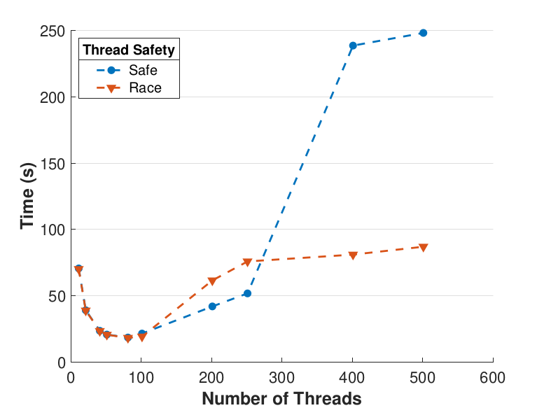
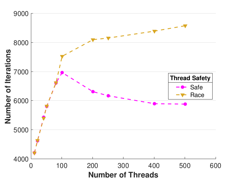
Figure 6 compares Safe and Race calculation times and number of iterations. Calculation times and average iteration counts are similar for thread counts up to 81, but behavior diverges beyond that. For thread counts 101 through 501, Race requires more iterations, perhaps to compensate for threads reading and computing with inaccurate 𝑥 vectors. Despite this, Figure 6(a) shows that Race is still quicker for the largest thread counts, perhaps because threads do not use locks to access data and eliminate that overhead cost. Figure 6(a) also shows that perhaps locks are not too costly for intermediate thread counts 101, 201, and 251, where Safe outperforms Race in terms of calculation time.
|
|
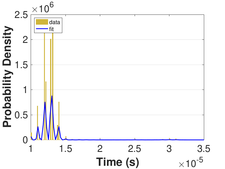
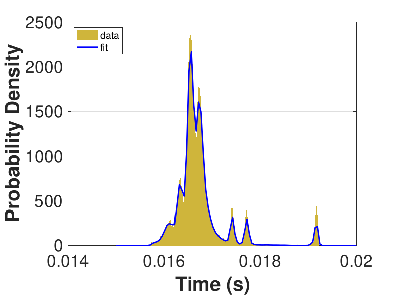
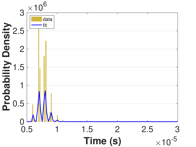
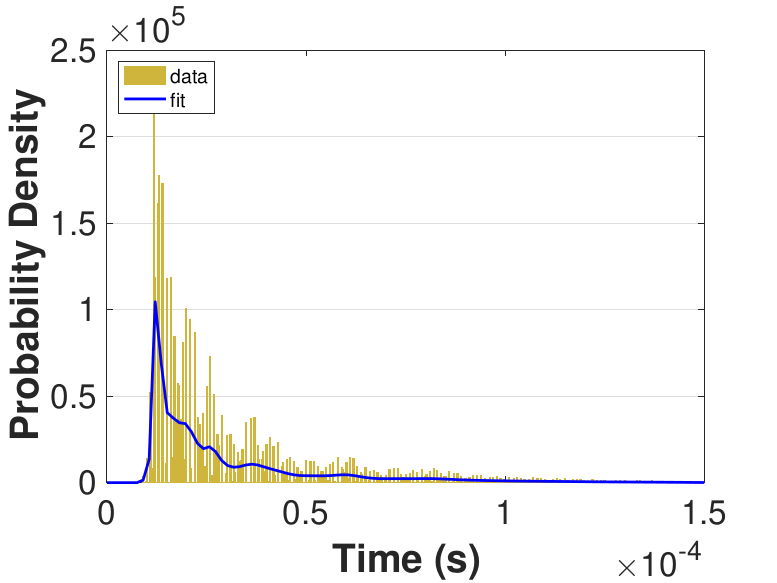
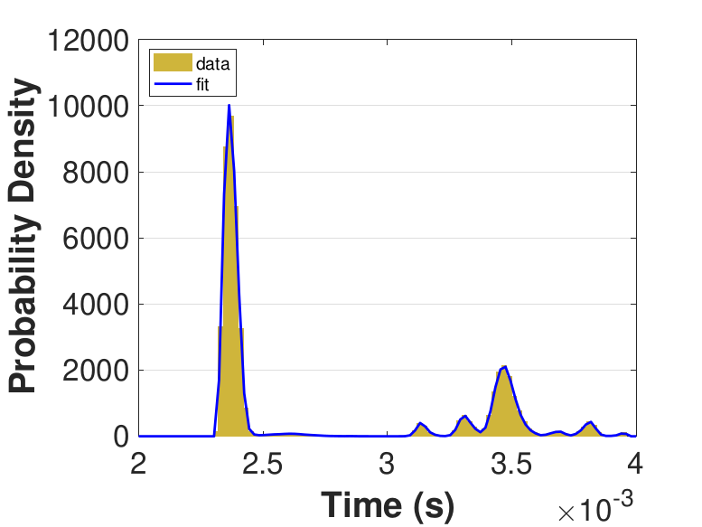
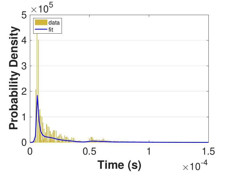
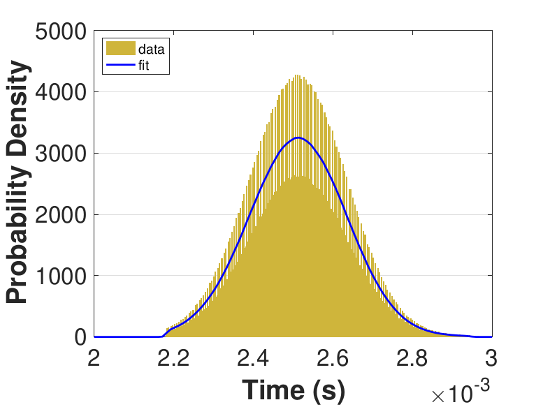
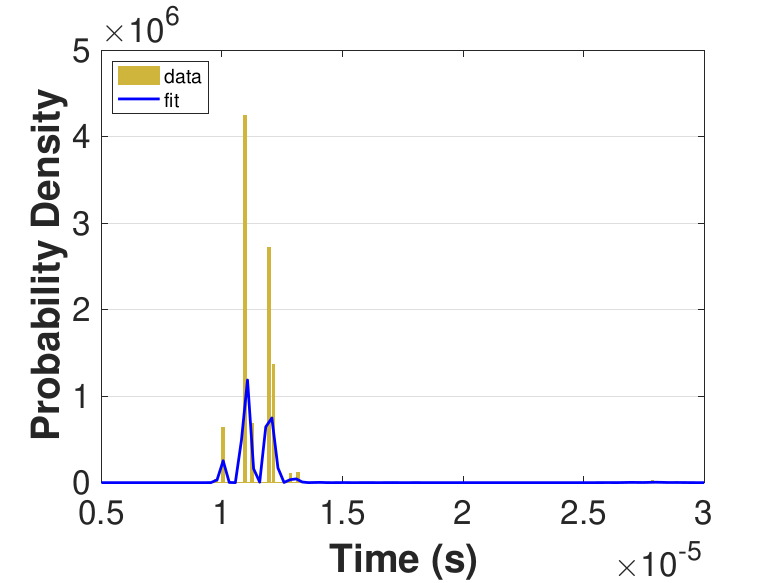
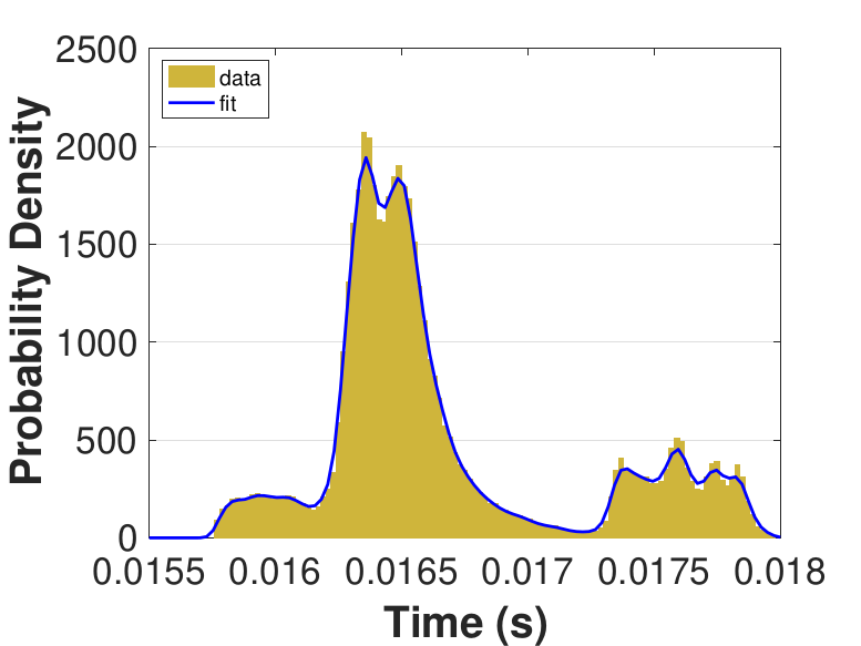
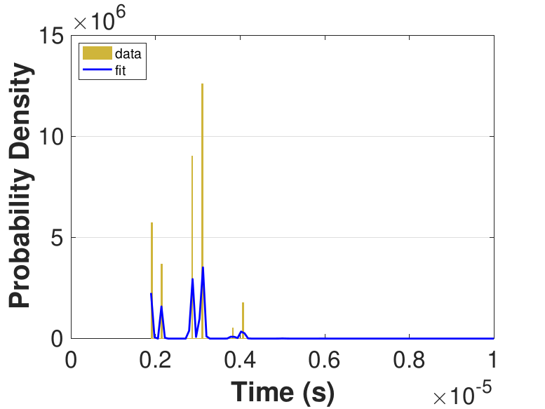
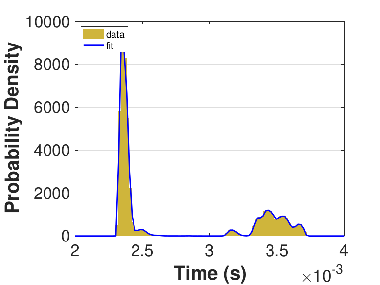
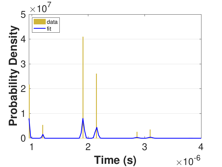
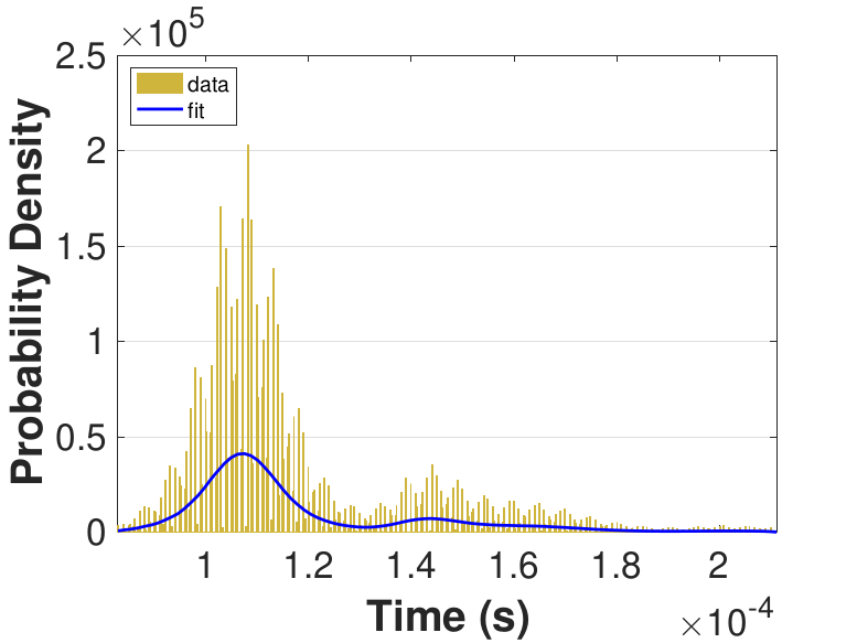
Both Safe and Race were executed over several trials and varying thread counts on the experimental HPC platform. For each trial, the times for a thread to access the solution in shared memory (Line 6 of Algorithm 3), compute the relaxation for the rows assigned to it (Line 11), and to update the solution in shared memory (Line 13) were captured. This data was used to generate MATLAB® kernel probability density functions for modeling the amount of time a thread takes to complete a copy, compute, or update operation. These distributions may be used in the simulation framework as an input parameter, for the generation of random variables corresponding to key operational times in the HPC architecture. Algorithm 2 demonstrates the use of a time distribution in the framework. Thread counts of 11, 21, 41, 81, 101, 201, 251, and 401 were used to collect data for the generation of distributions, some of which are in Figure 7 and Figure 8. For 201 threads, Safe in Figure 7(d) and Figure 7(f) shows the tendency of locks to stratify copy and update times, compared with Race in Figure 8(d) and Figure 8(f), which are less uniform. These findings are mirrored in Table 1, which provides mean times for each of the three operations that were benchmarked in this implementation, for Safe and Race. Race copy and update times are slightly or significantly quicker than comparable Safe times. Compute times typically dominate total iteration time, except for Safe copy and update times for threads 201, 251, and 401. Table 1 shows that increasing the number of threads decreases Race copy, compute, and update times until cores are sufficiently over-subscribed: at 201 threads, these operations have become significantly more costly, as compared with 101 threads. This cost may be attributed to thread context switching. Compute times for Safe do not increase with higher thread counts because thread behavior is controlled explicitly using locks. These statistics can be used to validate the performance of the time distributions, so that the framework provides results comparable to the HPC hardware.
| Threads | Safe | Race | ||||
|---|---|---|---|---|---|---|
| Copy (10−5s) |
Compute (10−4s) |
Update (10−6s) |
Copy (10−5s) |
Compute (10−4s) |
Update (10−6s) |
|
| 11 | 1.28 | 167.00 | 7.76 | 1.15 | 167.00 | 2.79 |
| 21 | 1.31 | 84.30 | 6.98 | 1.17 | 83.60 | 1.96 |
| 41 | 1.38 | 43.00 | 7.09 | 1.23 | 43.10 | 1.63 |
| 81 | 2.98 | 27.30 | 20.60 | 1.43 | 27.20 | 1.79 |
| 101 | 36.70 | 23.40 | 357.00 | 1.64 | 25.20 | 1.79 |
| 201 | 251.00 | 15.30 | 2500.00 | 11.80 | 74.30 | 4.33 |
| 251 | 345.00 | 13.30 | 3440.00 | 16.60 | 90.90 | 4.55 |
| 401 | 1880.00 | 8.23 | 18,700.00 | 20.20 | 91.60 | 4.52 |
|
|
|
|
|
|
|
|
|
|
|
|
|
|
|
|
|
|
Implementation 2: Finite Difference Jacobi Solver
This second implementation performs the Jacobi relaxation on the grid directly using the neighboring points required by the 5-point stencil as opposed to explicitly forming the matrix 𝐴, and in a sense implements a matrix-free solution. For this implementation, the Laplacian was discretized over a 600 × 600 grid with boundary conditions set according to Table 2.
| 0 | 100 | … | … | 100 | 0 |
| 75 | XXX | … | … | XXX | 50 |
| ⋮ | XXX | … | … | XXX | ⋮ |
| ⋮ | XXX | … | … | XXX | ⋮ |
| 75 | XXX | … | … | XXX | 50 |
| 0 | 0 | … | … | 0 | 0 |
The implementation used here stems from code provided by (Hager & Wellein, 2010); similar code solves a three dimensional discretization of the Laplacian in the study featured in (Bethune, Bull, Dingle, & Higham, 2011) and (Bethune, Bull, Dingle, & Higham, 2014). The routine solves a heat diffusion problem, in which a two-dimensional heated plate has Dirichlet boundary-condition temperatures. Two matrices, 𝑢0 and 𝑢1, store grid point values that each thread reads, e.g., from 𝑢1, to compute newer values to write, e.g., to 𝑢0. As the method is asynchronous, each thread independently determines which matrix stores its newer 𝑢(𝑡+1)(𝑖, 𝑗) values and older 𝑢(𝑡)(𝑖, 𝑗) values. For an 𝑁 + 2 by 𝑁 + 2 grid, each thread solves for 𝑁2 grid points divided by 𝑛 processing elements, such that the grid is evenly divided along the y-axis. When a thread copies grid point values above or below its domain for the computation, OpenMP® locks are employed to ensure that data is safely captured from a single iteration. Further, locks are used when updating values on domain boundaries. Each thread 𝑝𝑛 computes its local residual value every 𝑘th iteration, which it contributes to the global residual value using an OpenMP® atomic operation, such that it adds the local residual from the current iteration and subtracts the local residual from the previous iteration. A single thread checks for convergence with an atomic capture operation, and updates a shared flag variable if the criterion is satisfied. Pseudocode for this implementation is provided in Algorithm 4, where bold upper-case text indicates that OpenMP® locks are employed. Locks are used only with interior boundary rows, meaning they are unnecessary for the first and last rows in the domain.
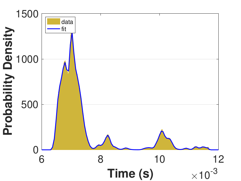
In this implementation, data was collected only for the time to complete an iteration. Thread counts of 10, 25, 50, 75, 100, and 150 were used in these series of experiments. The average total iteration time for the varying.
Algorithm 4 OpenMP Implementation 2
1:Input: Initial guess for , processing elements
2:Output: Solution vector
3:Assign rows to each processing element,
4:for parallel each processing element in do
5:while residual norm tolerance do
6:for row index do
7:if AND OR then
8:COPY neighbor or boundary row values for
9:end if
10:Compute
11:if AND OR then
12:UPDATE own boundary row values in shared memory with
13:end if
14:end for
15:end while
16:end for
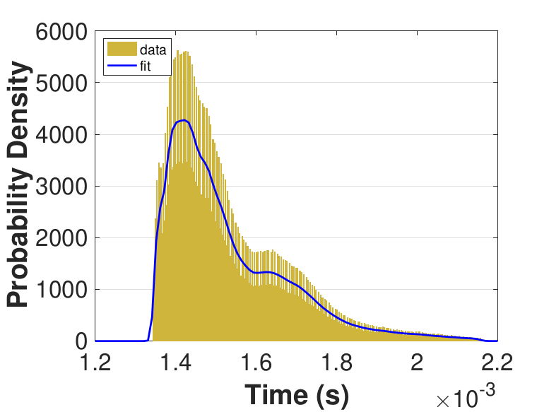
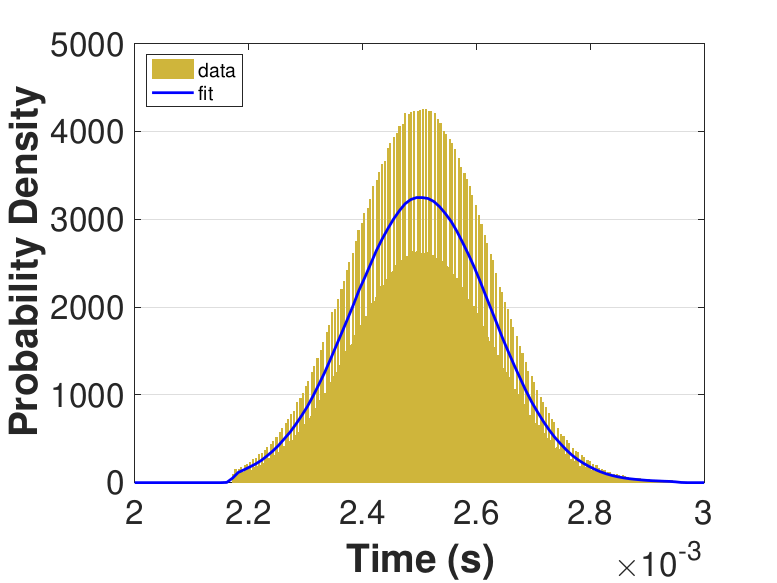
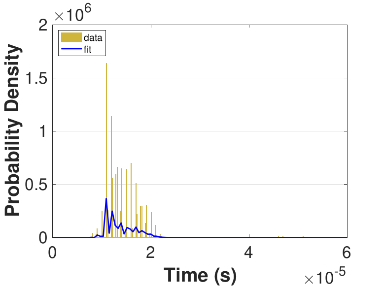
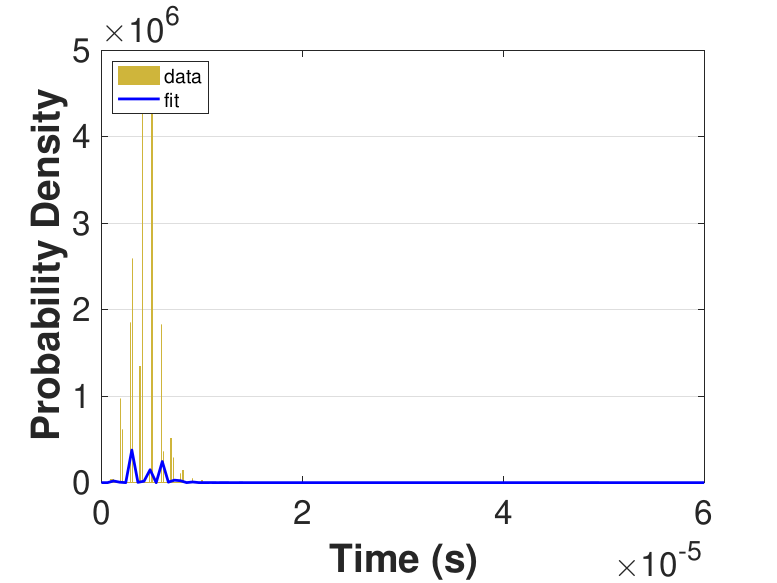
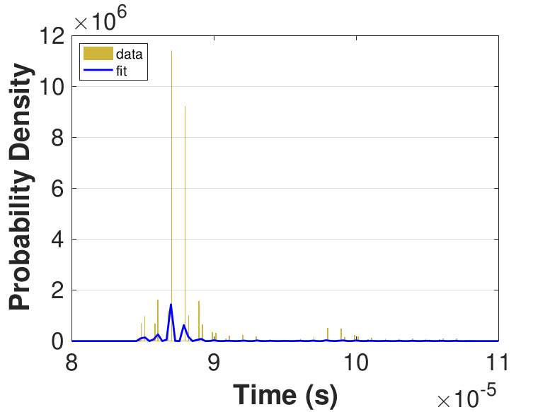
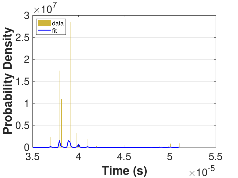
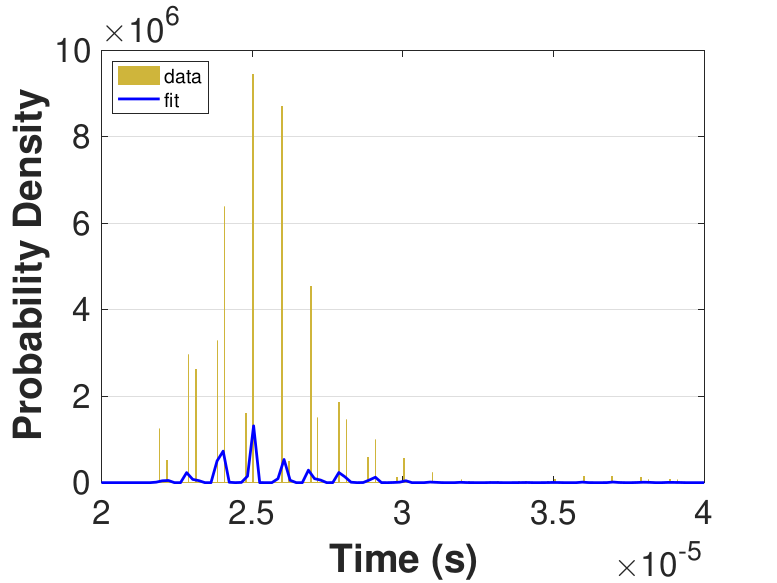
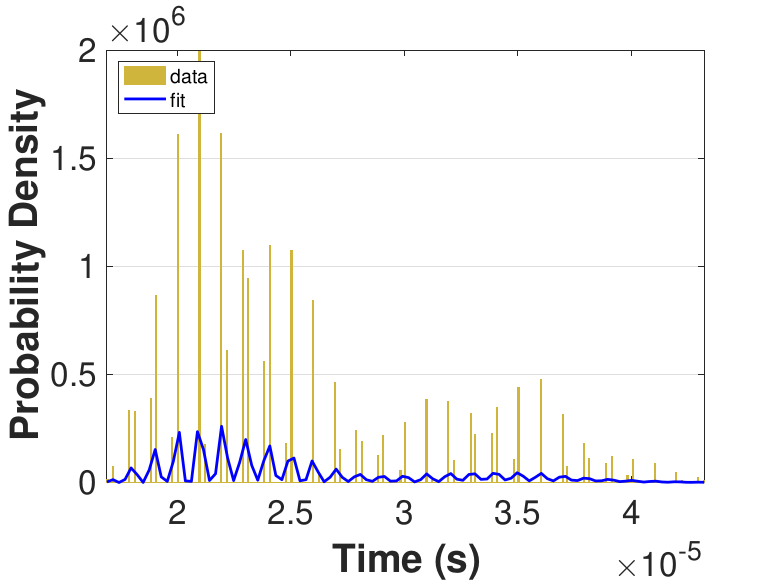
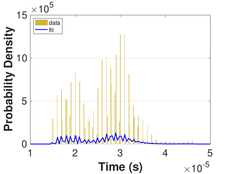
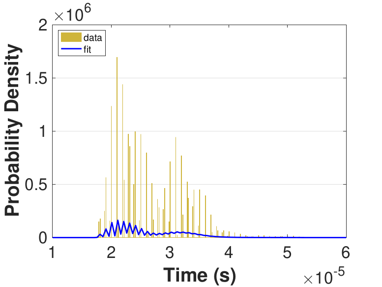
Figure 9 provides histograms and kernel fits for each of the thread counts. Table 3 and Figure 9 show that with increasing thread count, mean iteration time decreases, but iteration times variance increases. This increase in iteration time variation may result from increased opportunities for lock collisions with greater thread counts.
|
|
|
|
|
|
Since this implementation is even more compute bound than the first one, Table 3 shows a general decrease in the time for each iteration as the thread count is increased. While there is no inflection point evident in the data presented in Table 3, compared to Race in Table 1, Table 3 still suggests that once the number of threads outnumbers physical cores, performance gains diminish. For denser matrices, or for different applications on different systems, these trends could change as the memory-based activities become relatively more expensive. The finite difference discretization of the Laplacian is a very sparse matrix that does not require much data movement.
| Threads | Mean (10−5s) |
Std. (10−6s) |
|---|---|---|
| 10 | 8.86 | 3.87 |
| 25 | 3.92 | 2.08 |
| 50 | 2.55 | 2.34 |
| 75 | 2.53 | 5.80 |
| 100 | 2.61 | 5.95 |
| 150 | 2.64 | 5.76 |
Implementation Comparison
The Safe variant of the first implementation incurs significant overhead costs for 𝑥 copy and update operations, as thread count increases, because each thread must copy the entire 𝑥 vector. In the second implementation, data shared between threads is differentiated and specific to domain location; therefore, specific locks may be used when copying and updating segments of the subdomain. Assuming an appropriate number of processing elements for a given grid, i.e., a thread has significantly more middle rows than boundary rows, copy operations, and the associated variability and costs, are minimal compared with compute operations. The Race implementation of the general solver eliminates much of the overhead cost from mutex locks, and convergence time is satisfactory for the given system. Implementation 2 is more constrained than Implementation 1, generalizing only to finite difference discretizations of partial differential equations over rectangular grids. Implementation 1 generalizes further to any sparse matrix, 𝐴 with which the Jacobi method can be used. According to Theorem 1, convergence will occur if the spectral radius of the iteration matrix, 𝐶, is less than 1. In the case of the Jacobi method, the iteration matrix is given by
Note that in the two dimensional discretization of the Laplacian, the spectral radius of the Jacobian is less than l, which says that both the synchronous and asynchronous variants of the Jacobi algorithm will converge. Note Race behavior is unknown for different problems and HPC systems.
The purpose of the two distinct implementations is to emphasize that the simulation framework proposed here can adapt to the behavior of different problems and platforms. The framework may be apdapted to any asynchronous iterative method through the process of collecting data representative of individual update times and using the resultant data to model the system in the framework.
Framework Validation
To validate the performance of the simulation framework when initialized with appropriate distributions, a case study utilizing output from Implementation 1 (see Section 5.1 for details) was considered. Data was collected for a smaller problem size only in order to facilitate the collection of data over a large number of runs. Specifically, the Laplacian was discretized over a 20 × 20 grid resulting in a matrix of size 400 × 400. Similarly to the process in Section 5.1, distributions were fit to the output of the OpenMP® implementation, and these distributions were used in the simulation framework to provide update times to the simulated processors that are reflective of the HPC hardware that the data was collected on. Output from the average of these runs is provided in Table 4. The leftmost column provides the number of threads that were used (or simulated), the middle column shows the average over multiple runs of the parallel implementation, and the rightmost column shows the average over multiple runs of the simulation generated by the simulation framework. In the case of this small problem, the similarity of actual and simulated run times helps to validate the model. Running multiple trials of larger problems in the framework is currently time-prohibitive, which is an issue that may be improved with framework implementation changes. Future work includes model validation for other problems and larger problems.
| Thread Count |
Run Average (s) |
Simulation Average (s) |
|---|---|---|
| 11 | 0.01 | 0.01 |
| 21 | 0.02 | 0.02 |
| 41 | 0.04 | 0.04 |
| 51 | 0.04 | 0.05 |
| 81 | 0.09 | 0.09 |
| 101 | 0.12 | 0.12 |
| 201 | 0.34 | 0.35 |
Framework Extension for Fault-Tolerance Requirements
The modular nature of this framework allows for extra functionality to be easily added to the framework itself that can be used to adapt the base algorithm to suit a specific set of requirements. With the projected increase of faults (see the references in Section 2), development of fault tolerant algorithms is an important endeavor. A block diagram showing the additional functionality dealing with fault-tolerance is shown in Figure 10. The new functionality is achieved by passing in another function handle that performs the fault tolerance check and recovery work.
The contents of the newly added Fault tolerance check module may be organized as follows: Each processor makes a call to find the global residual and rolls the state back to the previous known good state if the behavior of the residual is not as expected. See Section 6.2 for more details. Note that this strategy is not being advocated for due to its optimality, but is being shown as an example of how to extend the framework for algorithm development. Techniques such as monitoring the progression of the component-wise residuals (e.g., (Anzt, Dongarra, & Quintana-Ortí, 2015; Anzt, Dongarra, & Quintana-Ortí, 2016)) or only rolling back portions of the state vector (e.g., (Coleman & Sosonkina, 2017; Coleman & Sosonkina, 2018)) would probably be more computationally efficient.
Fault Model
For this part of the study, faults are modeled as perturbations similar to several recent studies (Coleman & Sosonkina, 2016b; Coleman, Sosonkina, & Chow, 2017; Stoyanov & Webster, 2015); the goal being producing fault tolerant algorithms for future computing platforms that are not too dependent on the precise mechanism of a fault (e.g., bit flip). Modifying the perturbation-based fault model described in (Coleman, Sosonkina, & Chow, 2017), a single data structure is targeted and a small random perturbation is injected into each component transiently. For example, if the targeted data structure is a vector 𝑥 and the maximum size of the perturbation-based fault is ε then proceed as follows: sample a random number 𝑟𝑖 ∈ (-ε, ε) , using a uniform distribution, and then set
for all values of 𝑖. The resultant vector is then perturbed away from the original vector 𝑥. Other similar perturbation-based fault models have sampled the components 𝑟𝑖 from different ranges. This can allow the creation of scenarios where some components are perturbed by large amounts, and some are only changed incrementally.
In this study, faults are injected into the asynchronous Jacobi algorithm following the perturbation based methodology described above. Due to the relatively short execution time of the asynchronous Jacobi algorithm on the given test problems, a fault is induced only once during each run, and the fault is designated to occur at a random iteration number before convergence. To be precise — since "iteration" loses some meaning in an asynchronous iterative algorithm — the fault is injected on a single simulated time before the algorithm terminates. It is not necessary for the program to have an update scheduled on the same simulated time for the fault to be injected.
Experiments with the Fault-Tolerance Module
Similar to the earlier results in the paper, this study covers the solution of the linear system resulting from a two-dimensional finite difference discretization of the Laplacian. Before presenting simulation results, it is important to note that faults, as modeled here, will not prevent the eventual solution of the linear system using the (asynchronous) Jacobi method. Since the spectral radius of the associated iteration matrix is strictly less than 1, it will converge for any initial guess 𝑥(0).
Since faults are assumed to only affect the memory storing the vector 𝑥 and are assumed to occur in a transient manner, if a fault occurs on iteration 𝐹 then the subsequent iterate, 𝑥(𝐹+1) can be taken to be the new starting iterate and eventual convergence is guaranteed due to the iteration matrix which has remained the same throughout the occurrence of the fault. This model can reflect the scenario where certain parts of the routine are designated to run on hardware with a higher reliability threshold, and other parts of the algorithm are allowed to run on hardware that may be more susceptible to the occurrence of a fault. This sandbox type design has been suggested as a possible means for providing energy efficient fault tolerance on future HPC environments (Bridges, Ferreira, Heroux, & Hoemmen, 2012; Hoemmen & Heroux, 2011; Sao & Vuduc, 2013).
While eventual convergence may be guaranteed, greatly accelerated convergence is possible through a simple checkpointing scheme. An example of such a scheme (as an extension of the asynchronous Jacobi simulation provided by Algorithm 2) is provided in Algorithm 5.
Algorithm 5 Asynchronous Jacobi simulation with checkpointing
1:Input: ; initial guess ; number of processing elements ; input random number distribution; checkpointing tolerance ; checkpointing frequency
2:Output: Solution vector
3:Assign processor update times by sampling from an appropriate random number distribution
4:Assign a part of to each processing element
5:Initialize to a large value
6:for , until convergence do
7:for each processing element, do
8:if then
9:for each element assigned to do
10:
11:end for
12:Retrieve a new update time by sampling from the input distribution
13:end if
14:end for
15:Inject a fault if appropriate
16:Calculate the residual as in Equation (3)
17:if then
18:
19:end if
20:if then
21:
22:end if
23:Check termination conditions
24:end for
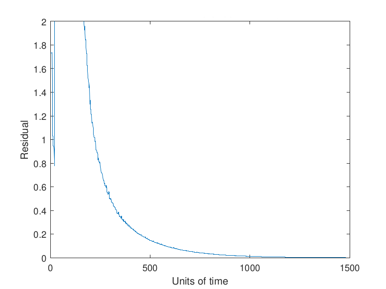
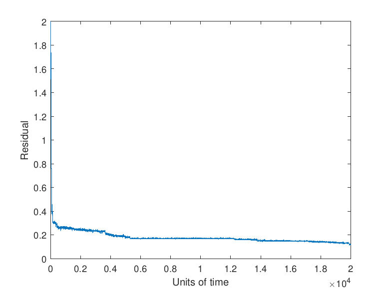
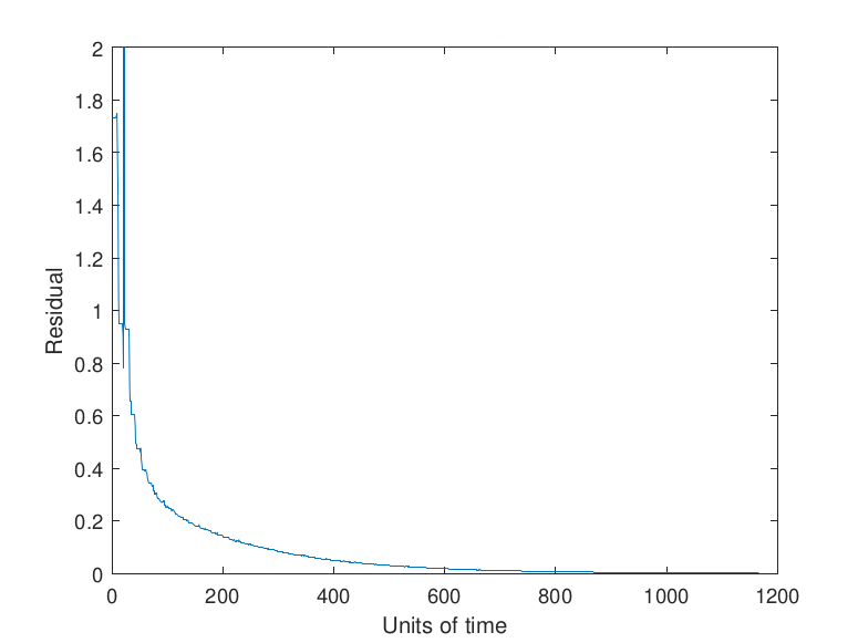
Note that the asynchronous nature of the iterative method means that a strict check on the decrease of the residual (i.e., expecting monotonic decrease) is not possible. In particular, the checkpointing tolerance α needs to be taken such that α > 1. However, the expected manifestation of faults as rare, transient events allows α to be taken fairly large. Taking α too large results in a fault having a substantial impact on the convergence rate of algorithm since large faults will be allowed to impact the algorithm with no correction. Conversely, taking α too small causes the algorithm to checkpoint more frequently than needed. Examples of the effects of a fault with different values selected for α are given by Figure 11.
|
|

|
|
Note in Figure 11 that no checkpointing results in a delay to convergence relative to the use of checkpointing with either α = 1 or α = 10. The size of the fault selected in this study, 𝑟𝑖 ∈ (-100, 100) , which may be reflective of an exponent or sign bit flip (Coleman & Sosonkina, 2018), results in the values α = 1 and α = 10 having the same performance since the error induced by the fault is sufficiently large that the new residual is more than α = 10 times the prior residual. Faults that induce a smaller error may be detected by certain values of α and not by others which would lead to differing performance.
The residual progress in the plot showing the effects of using α = 1 can be explained by the updates provided by certain simulated processing elements being rejected despite being necessary for the convergence of the algorithm. This can be seen in the small, momentary jumps in the progression of the residual visible in the other graphs. These rejections lead to stagnation in the progression of the algorithm and show why the value of α = 1 should not be selected for a checkpointing scheme for an asynchronous iterative method.
Conclusions and Future Work
This work has developed a framework that can be used to efficiently simulate the outcomes of asynchronous methods for future High Performance Computing environments. Given that asynchronous methods are notoriously difficult to study theoretically, their simulation is an invaluable tool for observing behavior and making quantitative and qualitative assertions. The modular and extensible nature of the framework proposed here allows for easy experimentation with modifications to a popular class of algorithms that finds uses in many areas of science and engineering.
The work presented was designed to show the ability of the framework to adapt to new algorithm variants, such as those capable of handling algorithm recovery in the presence of transient soft faults as was shown by example in Section 6.2.
The simulation framework presented here is extensible and flexible and is able to:
- admit a variety of asynchronous methods (i.e., beyond the simple Jacobi algorithm)
- incorporate different fault models and recovery techniques for the development of fault tolerant algorithms, and
- vary hardware parameters such as thread and processor counts and the performance of those parameters as governed by the timing distributions that are supplied.
In the future, the most obvious extension of the simulation framework is to add modules that allow it to be accurately used for experiments on either distributed or cloud-based computing environments. Additionally, it is planned to add features for optimization that could allow for the automation of the selection of the checkpointing tolerance as well as checkpointing frequency in the course of simulation. Adding the capability for the framework to take a range of parameters and find optimal values without direct input from the user could aid in the development of algorithms. Furthermore, the simulation framework is intended to be augmented with runtime simulation measurements, such those provided by Intel® Running Average Power Limit (RAPL) interface (Intel, 2016), to obtain simulated application execution traces in order to model application performance and energy consumption.
Acknowledgements
This work was supported in part by the Air Force Office of Scientific Research under the AFOSR award FA9550-12-1-0476, by the U.S. Department of Energy (DOE) Office of Advanced Scientific Computing Research under the grant DE-SC-0016564 and the Exascale Computing Project (ECP) through the Ames Laboratory, operated by Iowa State University under contract No. DE-AC00-07CH11358, by the U.S. Department of Defense High Performance Computing Modernization Program, through a HASI grant, the High Performance Computing facilities at Old Dominion University, and through the ILIR/IAR program at the Naval Surface Warfare Center — Dahlgren Division. Edmond Chow provided the MATLAB® script that evolved into part of the proposed simulation framework.
Footnotes
- Throughout the text, vector notation is occasionally adopted to emphasize when functions take all components of 𝑥 as opposed to a single component, such as 𝑥1.[back]
- Rulfo is a part of computing resources of the Department of Modeling, Simulation and Visualization Engineering at Old Dominion University.[back]
Bibliography
- Addou, A., & Benahmed, A.
(2005). Parallel Synchronous Algorithm for Nonlinear Fixed Point
Problems. International Journal of Mathematics and Mathematical
Sciences. 2005(19), 3175–3183.

- Anzt, H. (2012). Asynchronous
and Multiprecision Linear Solvers: Scalable and Fault-Tolerant
Numerics for Energy Efficient High Performance Computing (Doctoral dissertation, Karlsruher Institut für Technologie, Karlsruhe, Germany).

- Anzt, H., Chow, E., &
Dongarra, J. (2015). Iterative Sparse Triangular Solves for
Preconditioning. In Träff, J., Hunold, S., & Versaci, F. (eds) Euro-Par 2015: Parallel Processing. Euro-Par 2015 (pp. 650–661). Lecture Notes in Computer Science, vol 9233. Berlin, Heidelberg: Springer.
- Anzt, H., Dongarra, J., &
Quintana-Ortí, E.S. (2015). Tuning Stationary Iterative Solvers for
Fault Resilience. In Proceedings of the 6th Workshop on Latest
Advances in Scalable Algorithms for Large-Scale Systems (pp. 1:1–1:8). New York, NY: ACM.
- Anzt, H., Dongarra, J., &
Quintana-Ortí, E.S. (2016). Fine-Grained Bit-Flip Protection for
Relaxation Methods. Journal of Computational Science.
- Anzt, H., Luszczek, P.,
Dongarra, J., & Heuveline, V. (2012). GPU-Accelerated Asynchronous
Error Correction for Mixed Precision Iterative Refinement. In
Kaklamanis, C., Papatheodorou, T., & Spirakis, P.G. (eds) Euro-Par 2012 Parallel Processing (pp. 908–919). Lecture Notes in Computer Science, vol 7484. Berlin, Heidelberg: Springer.
- Asanović, K., Bodik, R.,
Catanzaro, B.C., Gebis, J.J., Husbands, P., Keutzer, K., Patterson, D.
A., Plishker, W.L., Shalf, J., Williams, S.W., & Yelick, K.A.
(2006). The Landscape of Parallel Computing Research: A View
from Berkeley (Report No. UCB/EECS-2006-183). Berkeley, CA: EECS
Department, University of California.
- Ashby, S., Beckman, P., Chen,
J., Colella, P., Collins, B., Crawford, D., Dongarra, J., Kothe, D.,
Lusk, R., Messina, P., Mezzacappa, T., Moin, P., Norman, M. Rosner, R.,
Sarkar, V., Siegel, A., Streitz, F., White, A., & Wright, M. (2010).
The Opportunities and Challenges of Exascale Computing: Summary
Report of the Advanced Scientific Computing Advisory Committee (ASCAC)
subcommittee. (Report No. Fall 2010). Washington, D.C.: U.S.
Department of Energy Office of Science.

- Avron, H., Druinsky, A. &
Gupta, A. (2015). Revisiting Asynchronous Linear Solvers: Provable
Convergence Rate through Randomization. Journal of the ACM,
62(6), 51:1–51:27.
- Baudet, G.M. (1978).
Asynchronous Iterative Methods for Multiprocessors. Journal of
the ACM, 25(2), 226–244.
- Benahmed, A. (2007). A
Convergence Result for Asynchronous Algorithms and Applications. Proyecciones (Antofagasta), 26(2), 219–236.
- Bertsekas, D.P., & Tsitsiklis, J.N. (1989). Parallel and Distributed Computation: Numerical Methods. Englewood Cliffs, NJ: Prentice-Hall.
- Bethune, I., Bull, J.M.,
Dingle, N.J., & Higham, N.J. (2011). Investigating the
Performance of Asynchronous Jacobi's Method for Solving Systems of
Linear Equations (Report No. 2011.82). Manchester: The University of Manchester.
- Bethune, I., Bull, J.M.,
Dingle, N.J., & Higham, N.J. (2014). Performance Analysis of
Asynchronous Jacobi's Method Implemented in MPI, SHMEM and OpenMP. International Journal of High Performance Computing Applications, 28(1), 97–111.
- Boyd, S., Parikh, N., Chu, E.,
Peleato, B., & Eckstein, J. (2011). Distributed Optimization and
Statistical Learning via the Alternating Direction Method of
Multipliers. Foundations and Trends in Machine Learning, 3(1),
1–122.
- Bridges, P.G., Ferreira, K.
B., Heroux, M.A., & Hoemmen, M. (2012). Fault-Tolerant Linear
Solvers via Selective Reliability. arXiv preprint
arXiv:1206.1390.
- Buyya, R. & Murshed, M.
(2002). Gridsim: A Toolkit for the Modeling and Simulation of
Distributed Resource Management and Scheduling for Grid Computing. Concurrency and Computation: Practice and Experience, 14(13–15), 1175–1220.
- Calheiros, R.N., Ranjan, R.,
Beloglazov, A., De Rose, C.A.F., & Buyya, R. (2011). CloudSim: A
Toolkit for Modeling and Simulation of Cloud Computing Environments and
Evaluation of Resource Provisioning Algorithms. Software:
Practice and Experience, 41(1), 23–50.
- Calheiros, R.N., Ranjan, R.,
De Rose, C.A.F., & Buyya, R. (2009). Cloudsim: A Novel Framework for
Modeling and Simulation of Cloud Computing Infrastructures and Services.
arXiv preprint arXiv:0903.2525.
- Cappello, F., Geist, A.,
Gropp, B., Kale, L., Kramer, B., & Snir, M. (2009). Toward Exascale
Resilience. International Journal of High Performance Computing
Applications, 23(4), 374–388.
- Cappello, F., Geist, A.,
Gropp, B., Kale, L., Kramer, B., & Snir, M. (2014). Toward Exascale
Resilience: 2014 update. Supercomputing Frontiers and
Innovations, 1(1).
- Casanova, H. (2001). Simgrid: A
Toolkit for the Simulation of Application Scheduling. In Proceedings
of the First IEEE/ACM International Symposium on Cluster Computing and
the Grid (pp. 430–437). Piscataway, NJ: IEEE Press.
- Casanova, H., Legrand, A.,
& Quinson, M. (2008). Simgrid: A Generic Framework for Large-Scale
Distributed Experiments. In Proceedings of the Tenth
International Conference on Computer Modeling and Simulation (UKSIM
2008) (pp. 126–131). Piscataway, NJ: IEEE Press.
- Chazan, D., & Miranker, W.
(2014). Chaotic Relaxation. Linear Algebra and its Applications, 2(2), 199–222.
- Cheung, Y.K. & Cole, R.
(2016). A Unified Approach to Analyzing Asynchronous Coordinate Descent
and Tatonnement. arXiv preprint arXiv:1612.09171.
- Chow, E., Anzt, H., &
Dongarra, J. (2015). Asynchronous Iterative Algorithm for Computing
Incomplete Factorizations on GPUs. In Kunkel, J., & Ludwig, T. (eds)
High Performance Computing. ISC High Performance 2015. Lecture
Notes in Computer Science, vol 9137. Cham: Springer.
- Chow, E., & Patel, A.
(2015). Fine-Grained Parallel Incomplete LU Factorization. SIAM
Journal on Scientific Computing, 37(2), C169–C193.
- Coleman, E.C., Jamal, A.,
Baboulin, M., Khabou, A., & Sosonkina, M. (2018). A Comparison of
Soft-Fault Error Models in the Parallel Preconditioned Flexible GMRES.
In Wyrzykowski, R., Dongarra, J., Deelman, E., Karczewski, K. (eds) Parallel Processing and Applied Mathematics. PPAM 2017. (pp. 36–46). Lecture Notes in Computer Science, vol 10777. Cham: Springer.
- Coleman, E.C., & Sosonkina, M. (2016a). A Comparison and Analysis of Soft-Fault Error Models using FGMRES. In Proceedings of the 6th Annual Virginia Modeling, Simulation, and Analysis Center Capstone Conference (pp. 135–142). Norfolk, VA: Virginia Modeling, Simulation, and Analysis Center.
- Coleman, E.C., & Sosonkina,
M. (2016b). Evaluating a Persistent Soft Fault Model on Preconditioned
Iterative Methods. In Proceedings of the 22nd Annual
International Conference on Parallel and Distributed Processing
Techniques and Applications (pp. 98–104). Athens: The Steering
Committee of The World Congress in Computer Science, Computer
Engineering and Applied Computing (WorldComp).
- Coleman, E.C., & Sosonkina, M. (2017). Fault Tolerance for Fine-Grained Iterative Methods. In Proceedings of the 7th Annual Virginia Modeling, Simulation, and Analysis Center Capstone Conference. Norfolk, VA: Virginia Modeling, Simulation, and Analysis Center.
- Coleman, E.C., & Sosonkina,
M. (2018). Self-Stabilizing Fine-Grained Parallel Incopmlete LU
Factorization. Sustainable Computing: Informatics and Systems,
(In Press).
- Coleman, E.C., Sosonkina, M.,
& Chow, E. (2017). Fault Tolerant Variants of the Fine-Grained
Parallel Incomplete LU Factorization. In Proceedings of the
25th High Performance Computing Symposium. San Diego, CA: Society for Computer Simulation International.
- Dongarra, J., Hittinger, J.,
Bell, J., Chacon, L., Falgout, R., Heroux, M., Hovland, P., Ng, E.,
Webster, A., & Wild, S. (2014). Applied Mathematics
Research for Exascale Computing (Report No. LLNL-TR-651000).
Livermore, CA: Lawrence Livermore National Laboratory.
- Dumitrescu, C.L., & Foster,
I. (2005). GangSim: A Simulator for Grid Scheduling Studies. In CCGrid 2005. IEEE International Symposium on Cluster Computing and the Grid (pp. 1151–1158, vol 2). Piscataway, NJ: IEEE Press.
- Elliott, J., Hoemmen, M., &
Mueller, F. (2015). A Numerical Soft Fault Model for Iterative Linear
Solvers. In Proceedings of the 24th International Symposium on
High-Performance Parallel and Distributed Computing (pp. 271–274). New York, NY: ACM.
- Frommer, A. & Szyld, D. B.
(2000). On Asynchronous Iterations. Journal of Computational
and Applied Mathematics, 123(1), 201–216.
- Gärtner, F.C. (1999).
Fundamentals of Fault-Tolerant Distributed Computing in Asynchronous
Environments. ACM Computing Surveys, 31(1), 1–26.
- Geist, A. (2011). What is the Monster in the Closet?. In Invited Talk at Workshop on Architectures I: Exascale and Beyond: Gaps in Research, Gaps in our Thinking (vol 2).
- Geist, A. (2012). Exascale Monster in the Closet. In 2012 IEEE Workshop on Silicon Errors in Logic-System Effects, Champaign-Urbana, IL, March (pp. 27–28). Piscataway, NJ: IEEE Press.
- Geist, A. (2016).
Supercomputing's Monster in the Closet. IEEE Spectrum. 53(3),
30–35.
- Geist, A., & Lucas, R.
(2009). Major Computer Science Challenges at Exascale. International
Journal of High Performance Computing Applications. 23(4), 427–436.
- Gerstenberger, R., Besta, M.,
& Hoefler, T. (2014). Enabling Highly-Scalable Remote Memory Access
Programming with MPI-3 One Sided. Scientific Programming,
22(2), 75–91.
- Hager, G., & Wellein, G.
(2010). Introduction to High Performance Computing for
Scientists and Engineers. Boca Raton, FL: CRC Press.
- Hoemmen, M., & Heroux, M.A.
(2011). Fault-Tolerant Iterative Methods via Selective
Reliability. vol 3.
- Hong, M. (2017). A Distributed,
Asynchronous and Incremental Algorithm for Nonconvex Optimization: An
ADMM Approach. IEEE Transactions on Control of Network Systems.
Piscataway, NJ: IEEE Press.
- Hook, J., & Dingle, N.
(2018). Performance Analysis of Asynchronous Parallel Jacobi. Numerical Algorithms. 77(3), 831–866.
- Intel (2016). Intel®
64 and IA-32 Architectures Developer's Manual. Volume 3B: System Programming Guide, Part 2.
- Iutzeler, F., Bianchi, P.,
Ciblat, P., & Hachem, W. (2013). Asynchronous Distributed
Optimization using a Randomized Alternating Direction Method of
Multipliers. In Decision and Control (CDC), 2013 IEEE 52nd
Annual Conference on (pp. 3671–3676). Piscataway, NJ: IEEE Press.
- Ortega, J.M., & Rheinboldt,
W.C. (2000). Iterative Solution of Nonlinear Equations in
Several Variables. Philadelphia, PA: SIAM.
- Saad, Y. (2003). Iterative
Methods for Sparse Linear Systems. Philadelphia, PA: SIAM.
- Sao, P. & Vuduc, R. (2013).
Self-Stabilizing Iterative Solvers. In Proceedings of the
Workshop on Latest Advances in Scalable Algorithms for Large-Scale
Systems (pp. 4:1–4:8). New York, NY: ACM.
- Snir, M., Wisniewski, R.W.,
Abraham, J.A., Adve, S.V., Bagchi, S., Balaji, P., Belak, J., Bose, P.,
Cappello, F., Carlson, B., Chien, A.A., Coteus, P., Debardeleben, N.A.,
Diniz, P.C., Engelmann, C., Erez, M., Fazzari, S., Geist, A., Gupta, R.,
Johnson, F., Krishnamoorthy, S., Leyffer, S., Liberty, D., Mitra, S.,
Munson, T., Schreiber, R., Stearley, J., & van Hensbergen, E.
(2014). Addressing Failures in Exascale Computing. International
Journal of High Performance Computing Applications. 28(2), 129–173.
- Srivastava, K., & Nedic, A.
(2011). Distributed Asynchronous Constrained Stochastic Optimization. IEEE Journal of Selected Topics in Signal Processing. 5(4), 772–790.
- Stoyanov, M. & Webster, C.
(2015). Numerical Analysis of Fixed Point Algorithms in the Presence of
Hardware Faults. SIAM Journal on Scientific Computing. 37(5),
C532–C553.
- Szyld, D.B. (1998). Different
Models of Parallel Asynchronous Iterations with Overlapping Blocks. Computational and Applied Mathematics. 17, 101–115.
- Tsitsiklis, J., Bertsekas, D.,
& Athans, M. (1986). Distributed Asynchronous Deterministic and
Stochastic Gradient Optimization Algorithms. IEEE Transactions
on Automatic Control. 31(9), 803–812.
- Venkatasubramanian, S., &
Vuduc, R.W. (2009). Tuned and Wildly Asynchronous Stencil Kernels for
Hybrid CPU/GPU Systems. In Proceedings of the 23rd
International Conference on Supercomputing (pp. 244–255). New York, NY: ACM.
- Wolfson-Pou, J., & Chow, E.
(2016). Reducing Communication in Distributed Asynchronous Iterative
Methods. Procedia Computer Science. 80, 1906–1916.
- Zhong, M., & Cassandras, C.
G. (2010). Distributed Asynchronous Deterministic and Stochastic
Gradient Optimization Algorithms. IEEE Transactions on
Automatic Control. 55(12), 2735–2750.
Copyright Information
 Copyright © 2018 Evan C. Coleman, Erik Jensen, Masha Sosonkina. This article is licensed under a Creative Commons Attribution 4.0 International License.